Having trained a model, it is natural to want to understand how it works. An intuitively appealing approach is to consider data samples that maximise the activation of a hidden unit, and to take the common input features of these samples as an indication of what that unit has learned to recognise. However, as we’ll see below, it is a misconception to speak of hidden units if:
- there is no non-linearity on the hidden layer;
- the weights connecting the layers are unconstrained; and
- the model is trained using (stochastic) gradient descent or similar.
In such a scenario, the hidden feature space must instead be considered as a whole.
Summary
Consider the task of factorising a matrix $ X $ as a product of matrices $ X \cong A^T B $ with some fixed inner dimension $ k $. The model parameters are pairs of matrices $ (A, B) $ with the appropriate dimensions, and the image of an input vector $ x $ on the hidden layer is given by $ Ax $. To consider this vector $ Ax $ in terms of hidden unit activations is to fix a co-ordinate system in the hidden feature space, and to measure the displacement of the vector along each co-ordinate axis. If $ E_1, \dots , E_k $ denote the unit vectors corresponding to the chosen co-ordinate system, then the displacements are given by the inner products
\begin{equation*} \langle Ax, E_i \rangle, \quad i = 1, \dots, k. \end{equation*}
We show below that if $ P $ is any rotation of the hidden feature space, then the model parameters $ (PA, PB) $ are just as likely as $ (A, B) $ to result in the factorisation of a fixed matrix $ X $ and that which of these occurs depends only on the random initialisation of gradient descent. Thus the hidden unit activations might just as likely have been given by
\begin{equation*} \langle (PA)x, E_i \rangle, \quad i = 1, \dots, k. \end{equation*}
The hidden unit activations given by 1 and 2 can be very different indeed. In fact, since $ P $ is an orthogonal transformation, we have
\[
\langle (PA)x, E_i \rangle = \langle Ax, P^T E_i \rangle, \quad i = 1, \dots, k
\]
(see e.g. here). Thus the indeterminacy of the model parameters, i.e. $ (A, B) $ vs. $ (PA, PB) $, might equivalently be thought of as an indeterminacy in the orientation of the co-ordinate system, i.e. the $ E_i $ vs. the $ P^T E_i $. The choice of orientation of co-ordinate basis is completely arbitrary, so speaking of hidden unit activations makes no sense at all.
The above holds more generally for $ P $ an orthogonal transformation of the hidden feature space, i.e. for $ P $ a composition of rotations and reflections.
Szegedy et al.
None of the above is new. For example, it was stated by Szegedy et al. in an empirical study of the interpretability of hidden units. We are demonstrating, step-by-step, a statement of theirs (which was about word2vec):
… word representations, where the various directions in the vector space representing the words are shown to give rise to a surprisingly rich semantic encoding of relations and analogies. At the same time, the vector representations are stable up to a rotation of the space, so the individual units of the vector representations are unlikely to contain semantic information.
Matrix factorisation and unit activation
Given a matrix $ X $ and an inner dimension $ k $, the task of matrix factorisation is to learn two matrices $ A $ and $ B $ whose product approximates $ X $:
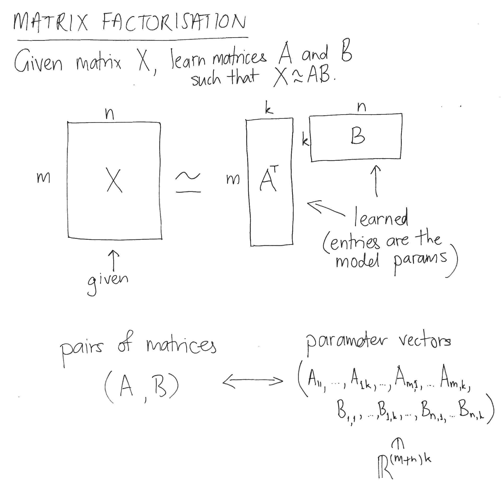
The parameter space consists of the entries of the matrices $ A $ and $ B $. The hidden feature space, on the other hand, is the k-dimensional space containing the columns of $ A $ and $ B $.
Error function
To train a matrix factorisation model using gradient descent, the model parameters are repeatedly updated using the gradient vector of the error function. An example error function $ E $ could be
\[
E_X (A, B) = \sum_{i, j} {(X_{i, j} – (AB)_{i,j})^2}.
\]
Notice that this choice of error function doesn’t depend directly on the pair of matrices $ (A, B) $, but rather only on their product $ AB $, i.e. only on the approximation $ AB $ of $ X $. This is true of any error function $ E_X $, because error functions depend only on inputs and outputs.
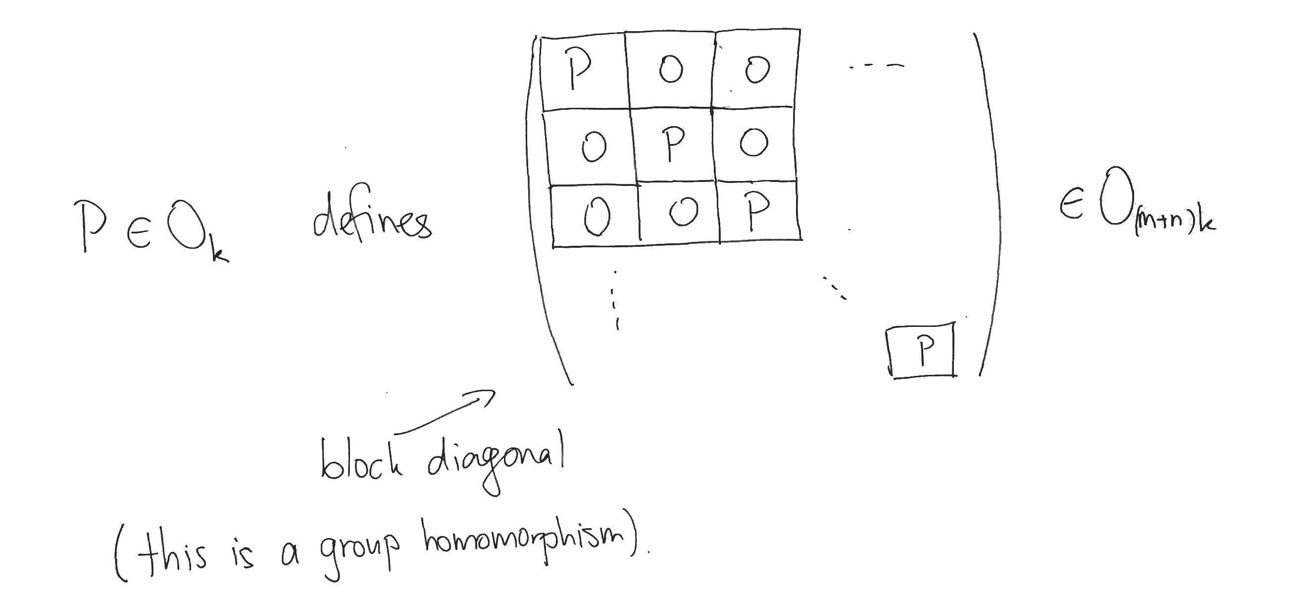
Orthogonal transformations of the hidden feature space
Recall that orthogonal transformations of a space are just compositions of rotations and reflections about hyperplanes passing through the origin. Considered as matrices, orthogonal transformations are defined by the property that their product with their transpose gives the identity matrix. Using this property, it can be seen that an orthogonal transformation of the hidden feature space defines an orthogonal transformation of the parameter space by acting simultaneously on the column vectors of the matrices. If $ O_k $ and $ O_{(m+n)k} $ denote the groups of orthogonal transformations on the hidden feature space and the parameter space, respectively, then:
Contour lines of the gradient
The effect of this block-diagonal orthogonal transformation on the parameter space corresponds to multiplying the matrices $ A $ and $ B $ on the left by the orthogonal transformation $ P $ of the feature space, i.e. it effects $ (A, B) \mapsto (PA, PB) $. Notice that $ (A, B) $ and $ (PA, PB) $ yield the same approximation to the original matrix $ X $, since:
\[
(PA)^T (PB) = (A^T P^T) (PB) = A^T (P^T P) B = AB.
\]
Thus $ E_X (A, B) = E_X (PA, PB) $, so the orthogonal transformations $ P $ of the hidden feature space trace out contour lines of $ E_X $ in the parameter space. Now the gradient vector is always perpendicular to the contour line, so the sequence of points in the parameter space visited during gradient descent preserve the orientation of the hidden feature space set at initialisation (see here, for example). So if gradient descent of $ E_X $ starting at the initial parameters $ (A^{(0)}, B^{(0)}) $ converges to the parameters $ (A, B) $, and you’d prefer that it instead converged to $ (PA, PB) $, then all you need to do is start the gradient descent over again, but this time with the initial parameters $ (PA^{(0)}, PB^{(0)}) $. We thus see that the matrices $ (A, B) $ that our matrix factorisation model has learned are only determined up to an orthogonal transformation of the hidden feature space, i.e. up to a simultaneous transformation of their columns.
Gradient descent methods
The above statements continue to hold in the case of stochastic gradient descent, where the error function $ E_X $ is not fixed but rather defined by varying mini-tasks (an instance being e.g. word2vec). Such error functions still don’t depend upon hidden layer values, so as above their gradient vectors are perpendicular to the contour lines traced out by the orthogonal transformations of the hidden layer. Thus the updates performed in stochastic gradient descent also preserve the original orientation of the feature space.
Initialisation
How likely is it that initial parameters, transformed via an orthogonal transformation as above, ever occur themselves as initial parameters? In order to conclude that the orientation of the co-ordinate system on the hidden layer is completely arbitrary, we need it to be precisely as likely. Thus if $ \pi $ denotes the probability distribution on the parameter space from which the initial parameters are drawn, we require
\[
\pi ( (P A^{(0)}, P B^{(0)}) ) = \pi ( (A^{(0)}, B^{(0)}) ),
\]
for any initial parameters $ ( A^{(0)}, B^{(0)} ) $ and any orthogonal transformation $ P $ of the hidden feature space.
This is not the case with word2vec, where each parameter is drawn independently from a uniform distribution. However, it remains true that for any choice of initial parameters, there will still be any number of possible orientations of the co-ordinate system, but for some choices of initial parameters there is less freedom than for others.
Appendix: What about GloVe?
GloVe performs weighted matrix factorisation with bias terms, so the above should apply. The weighting is just a modified error function, and the bias terms are not hidden features and so are left unmodified by its orthogonal transformations. Like word2vec, GloVe initialises each parameter with independent samples from uniform distribution, so there are no new problems there. The real problem with applying the above analysis to GloVe is that the implementation of Adagrad used makes the learning regime dependent on the choice of basis of the hidden feature space (see e.g. here). This doesn’t mean that the hidden unit activations of GloVe make sense, it just means that GloVe is less amenable to theoretical arguments like those above and needs to be considered empirically e.g. in the manner of Szegedy et al.