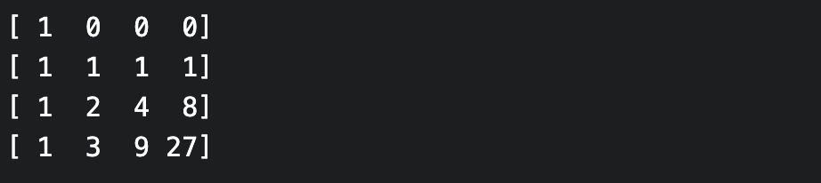
The Vandermonde matrix computes evaluations of polynomials from their coefficients via a matrix-vector product. The Vandermonde matrices are nested, i.e. each Vandermonde matrix is the principal submatrix of any larger Vandermonde matrix that uses (an extension of) the same sequence of evaluation points. For example, here is the (square) Vandermonde matrix for the evaluation points ; the Vandermonde matrix for is the x principal (i.e. top-left) submatrix:
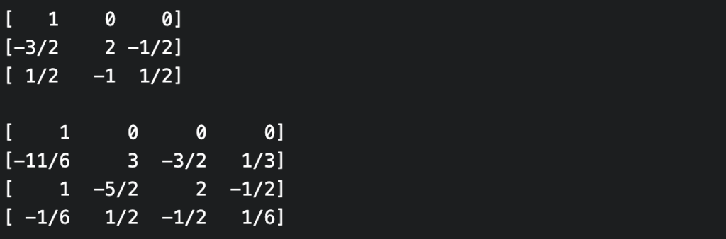
If the inverse Vandermonde matrix exists, then the inverse computation (from evaluations to coefficients, i.e. polynomial interpolation), can also be performed as a matrix-vector product (for the inverse of the Vandermonde matrix to exist, it must be square and the evaluation points must be distinct). Unfortunately, the inverse Vandermonde matrices are no longer “nested” in the above sense. For example, here are the inverse Vandermonde matrices for evaluation points and .
Who cares? Well, it would be nice if they were nested since then one could pre-compute a sufficiently large inverse Vandermonde matrix, and be able to interpolate any polynomial that came along. But it just isn’t so! However, for the particular case where the evaluation points are the non-negative integers (and indeed in many more general cases), the neatness can be restored using a certain triangular decomposition of the Vandermonde matrix and its inverse.
Let’s write for the Vandermonde matrix for the evaluation points . Then can be expressed as a product of an lower-triangular, diagonal and upper-triangular matrices , , and i.e. . Thus . It turns out that all of these factors form nested families in the sense above, e.g. is the principal x submatrix of any , while is the principal x submatrix of , and so on. Thus if we pre-compute then we’ll be able to interpolate any polynomial of degree at most (by selecting the appropriate principal submatrix of each factor, and then performing three matrix-vector multiplications).
Furthermore, the entries of (also of , , ) are given by pleasing and useful recursive formulae, and these can be used to increase the size of your precomputed matrices as required. For instance, and the identity is easily adapted to a recurrence on the that allows us to extend as needed. The diagonal entries of are given by (recurrence obvious) while the entries of are given by the (signed) Sterling numbers of the first kind via . These quantities satisfy the recurrence with boundary conditions and for all .
These formulae were first derived in Vandermonde matrices on integer nodes (Eisinberg, Franzé, Pugliese; 1998). Another useful (and freely available) reference is Symmetric functions and the Vandermonde matrix (Oruç & Akmaz; 2004) which deals with the case of -integer nodes (take in their Theorem 4.1 to obtain the formulae above).
Polynomials are formal sums. So in particular, is infinite-dimensional over , even if e.g. , the field with two elements. This is true even though e.g. is the zero function on , as you can check by substituting and for .
Polynomial functions are functions e.g. on the field itself (or, more generally, on some object that can be locally parameterized by the field). But let’s simply consider , the set of polynomial functions from the field to itself. is a ring with addition and multiplication given point-wise on function values. Any polynomial can be considered a polynomial function in the obvious manner, and this defines a surjection of rings: In the case where is a finite field, is a proper quotient of i.e. . To see this, consider the multiplicative group . Then , where . Therefore for any , and so for any . We’ve shown therefore that the non-zero polynomial is in , since it is maps to the zero function on . This is just the generalization of our observation for , above.
In fact, we’ve found a generator for the kernel, i.e. . One way to see this is to check that the polynomial functions defined by first monomials are linearly independent as functions on , which can be done using the Vandermonde matrix and the distinct non-zero field elements at your disposal. Another way to see this, since we are working over a finite field, is to simply count the elements of the quotient and of . There are clearly elements in the quotient, but what about ? It turns out that consists of all functions . To see this, given any function on , just use Lagrange interpolation to build yourself a polynomial of degree that matches the function at all points. There are functions , and so that’s the size of . Thus the quotient has the same number of elements as . But we have a chain of surjections so .
On the other hand, if the field is infinite, then is zero, i.e. polynomials over and polynomial functions on are isomorphic. To see this just show that the set of all monomials is linearly independent, using the Vandermonde matrix and the endless supply of distinct non-zero elements of .
The multivariate case is entirely analogous
All functions are polynomial functions. To see this, just mimic the Lagrange interpolation of the univariate case (it’s sufficient to convince yourself that, given any point in , you can write down a polynomial function that takes the value 1 there, and the value 0 everywhere else). Thus, since there are functions , this is the size of , the ring of polynomial functions on .
Now write for the obvious surjection of rings. Then it follows immediately from the univariate case that we have an inclusion of ideals Now notice that the quotient has elements. This is the same number as above, and so we conclude that we’ve already found the full kernel, i.e.
Here is a nice simple example of bilinear pairing on an elliptic curve over a finite field. Different sorts of pairings exist – here we’ll construct a pairing that coincides with the Weil pairing. For simplicity, our construction will avoid talking about divisors on algebraic curves.
Consider the elliptic curve over defined by the equation There are nine solutions: The identity element is a point at infinity corresponding to the vertical axis (it is a point of the projective plane). All the other points are elements of the affine plane . These nine points form a group which we’ll denote by .
We can check that for any , we have . The most elementary way to check this is by direct calculation: we need to check that for each point . Recalling the diagrammatic rule for computing , we need to draw the tangent to the curve at , and then find the other point of intersection with the curve (it turns out this geometric interpretation of point doubling works over prime fields as well). So let’s calculate the slope of the tangent at each point : This gives us the following diagram:
The dashed blue lines indicate the tangents to the curve at each point. Check for yourself that if you follow any of these tangents (remembering to wrap around to the opposite side when you get to an edge!) then you don’t hit any other points, i.e. the point of tangency is the only point of the elliptic curve on the tangent line, meaning that the “other” point of intersection must be itself (this means it’s an intersection of “higher order”). So is equal to the reflection of through the line , i.e. , and so , as claimed.
In fact, it turns out that as groups; you can construct such an isomorphism yourself by setting e.g. and and taking these as the generators of the two copies of in the direct product. Note that this choice of isomorphism is not canonical (i.e. there is nothing to justify this particular choice) but that’s fine for our purposes. All we really need is that any has a unique expression as a -linear combination of our chosen generators .
We are finally in a position to define a bilinear pairing. There are various types of pairings. Here, we’ll construct the Weil pairing. Let be an abelian group, written multiplicatively. We want a map that is bilinear, i.e. for all , and alternating, i.e. Some further properties follow immediately. For example, using that , it follows from bilinearity that and from this last property and the fact that for all , it follows that and so we might as well take to be the group of third roots of unity over . Note in fact contains all its third roots of unity, since modulo .
So how many alternating, bilinear forms can be there be on ? Up to a choice of third root of unity, just one! To see this, just use the bilinearity and alternation properties to check that i.e. all such forms are given by some third root of unity raised to the power of the determinant of the matrix of coefficients. And on the other hand, since we know that the determinant is an alternating multilinear function on matrix rows, we see that this definition really does give us an alternating bilinear form on . From uniqueness, we know that this pairing must in fact coincide (up to choice of root of unity) with the Weil pairing of our elliptic curve, since it too is alternating and bilinear.
What about the general case? The Weil pairing is defined on the “-torsion” of an elliptic curve, i.e. the subgroup of points such that . In our example, and the -torsion subgroup coincides with the entire group (this is rarely true). On the other hand, the group isomorphism holds in general, with the caveat that you’ll likely need to take an extension field (not a prime field) as your base field.
Is this construction useful? While the above construction might be instructive, it isn’t useful. In order to prove useful things about the pairing, the divisor-theoretic construction is much more useful, since it allows us to call on the theory of algebraic curves (and in fact this is needed to even prove that is a group!). Furthermore, in order to actually calculate a Weil pairing using the determinant construction, it is necessary to express an arbitrary as a linear combination of the chosen generators (and this problem would be hard even if there was just one generator: that’s the discrete logarithm problem!). So there are good reasons for the definition of the Weil pairing in terms of divisors, after all.
It should also be noted that the (divisor-theoretic) construction of the Weil pairing is canonical, not requiring a choice of basis for nor a choice of primitive root of unity.
Addendum #1: as an alternative to the slope/tangent method above for visually checking that each point has order , you can check instead that the Hessian determinant of the homogenisation of the equation defining the elliptic cruve vanishes at each point, i.e. show that each point is a point of inflection. See Silverman’s The Arithmetic of Elliptic Curves, exercise III.3.9.
Addendum #2: The example above has been chosen so that everything can be calculated by hand. To work with other examples, or to check your work, Magma is a great help. Here is some example code for the above calculations, which you can plug into the online calculator:
K := GF(7);  // the finite field with 7 elements

// The EC with equation y^2 = x^3 + 0*x + 2 over K
E := EllipticCurve([K | 0, 2]);
print E, "\n";

print "Number of points on the curve", #E, "\n";

// Creation of a point with given projective coordinates
P := E ! [6, -1, 1];

print "The order of each element:";
for P in Points(E) do
    print "Element", P, "has order", Order(P);
end for;
print "\n";

print "Point doubling:";
for P in Points(E) do
    print "2", P, "=", P+P;
end for;
print "\n";

print "Find a decomposition of E as a product of finite cyclic groups:";
AbelianGroup(E);
print "\n";

print "Calculate the Weil pairing:";
for P in Points(E) do
    for Q in Points(E) do
        P, "paired with", Q, "=", WeilPairing(P, Q, 3);
    end for;
end for;
Here is a first example of an elliptic curve over a finite field where you can work everything out by hand.
Consider the elliptic curve defined by the equation over the field . Multiplying out the right hand side, we see that (over ), the right hand side (“RHS”) is . So our equation is not in Weierstrass form, but that’s fine. It’s still defines an elliptic curve. Note that we know immediately that it is non-singular, since the roots of the RHS are distinct.
It’s easy to find all the solutions to our equation by hand – just consider each possible value for , calculate the RHS, and set , if such exist. So we first need to know which values in are squares:
Thus the points on our elliptic curve are The point is the solution at infinity: this is the one extra solution that arises when the equation defining the elliptic curve is homogenized, and solutions in the projective plane are permitted. The other solutions live in the “affine” plane.
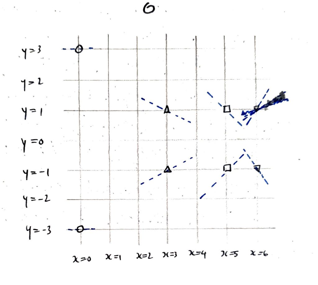
The nice thing about working over an unextended finite field like is that it is still “1-dimensional”, so the affine solutions can be depicted on a 2-dimensional diagram like the following:
Fortunately, the familiar geometric description of the group operation on elliptic curves in terms of line intersections still works (why?). That is, any two points can be added by drawing a line through them, finding the third point of intersection, and reflecting through the line , and the point corresponds to the vertical direction and is the identity element of the group.
For example, it is immediate from this rule that . Remembering that lines wrap-around our diagram (which is actually a torus), what do you think is equal to? (Hint: it’s the next letter of the alphabet).
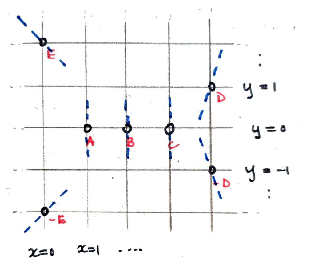
As in the case over :
If a vertical line passes through two distinct affine points such as and , then (since it also intersects with in the projective plane) these points are inverses of one another w.r.t. the group operation. (We’ve labelled to reflect this.)
If a vertical line hits a single affine point (e.g. the line ) then this point is its own inverse.
Thus are all group elements of order 2.
Amusingly, the geometric rule for point doubling using tangents still works, as well. The slope of the tangent at a point on our elliptic curve can be calculated in the usual way. These slopes are depicted on our diagram with dashed blue lines. Following these tangents, you can immediately verify that and so have order as group elements.
The orders of our group elements are enough to conclude that our group (call it ) is isomorphic to . Indeed, since and (to check, just follow the lines!) we have that is an isomorphism of groups
I prepared the following one-page overview of the short-time Fourier transform for a recent talk, perhaps it’ll be useful to others. For justification of e.g. the conjugate symmetry of the Fourier coefficients or a discussion of aliasing, see here.
We aim to identify the assumptions that are implicit in the sampling of a continuous-time signal and in the subsequent application of the discrete Fourier transform (DFT). In particular, we consider the following questions:
When does the sampling of periodic continuous-time signal result in a periodic discrete-time signal?
When the resulting discrete-time signal is periodic, what is its frequency in samples/second?
Which continuous-time frequencies coincide in discrete time, and what does the “frequency spectrum” in discrete-time look like?
To which periodic discrete-time signals can the discrete Fourier transform be applied to without losing information?
We furthermore show that the DFT interchanges point-wise and convolution products in the time- and frequency- domains, and thereby express the DFT to Pontryagin duality for finite cycle groups.
I talked about the above (skipping many details!) at a recent talk.
Below are the notes I made to prepare for a short talk given at our seminar on learning distance metrics, and the Mahalanobis distances in particular. We show that the Mahalanobis distances can be parameterised by the positive semidefinite (PSD) matrices or alternatively (in a highly redundant way) by all matrices. The set of PSD matrices is convex, but in order to perform gradient descent to optimise the objective function, we need to perform a costly projection after each update involving the singular value decomposition.
We note along the way that a Mahalanobis distance is nothing more than the Euclidean distance after applying a linear transform to the data.
The example of the 2×2 PSD matrices is worked out in detail here.
What’s here documents my first steps. What I really discovered is that metric learning is a research domain in its own right, and that a great deal of work has been done. There is an excellent survey by Bellet et al. (2013) that covers everything I have said in the first two of its sixty pages.
Recall that a symmetric matrix is called positive semidefinite (“PSD”) if, for any , we have . Positive semidefinite matrices occur, for instance, in the study of bilinear forms and as the Gram (or covariance) matrices in probability theory. In the case where , the space of symmetric matrices is 3-dimensional, and we can actually draw the subset of all positive semidefinite matrices – it looks like the bow of a ship.
It is clear that in the case illustrated below, the PSD matrices form a convex subset. It is easy to show this in general, by observing that the set of all PSD matrices is closed under addition and multiplication by non-negative scalars. The convexity of this set is crucial for the fitting of Mahalanobis distances in metric learning, which is how I got interested PSD matrices in the first place.
Below are the notes I prepared for a talk that I gave at our seminar on limiting distributions for (finite-state, time-homogeneous) Markov chains, drawing on PageRank as an example. We see in particular how the “random teleport” possibility in the PageRank random walk algorithm can be motivated by the theoretical guarantees that result from it: the transition matrix is both irreducible and aperiodic, and iterated application of the transmission matrix converges more rapidly to the unique stationary distribution.
Update: that the limit of the average time spent is the reciprocal of the expected return time can be proved using the renewal reward theorem (thank you Prof. Sigman!)
We show below that vectors drawn uniformly at random from the unit sphere are more likely to be orthogonal in higher dimensions.
In information retrieval and other areas besides, it is common to use the dot product of normalised vectors as a measure of their similarity. It can be problematic that the similarity measure depends upon the rank of the representation, as it does here — it means, for example, that similarity thresholds (for relevance in a particular situation) need to be re-calibrated if the underlying vectorisation model is retrained e.g. in a higher dimension.
Question
Does anyone have a solution to this? Is there a (of course, dimension dependent) transformation that can be applied to the dot product values to arrive at some dimension independent measure of similarity?
I asked this question on “Cross Validated”. Unfortunately, it has attracted so little interest that it has earned me the “tumbleweed” badge!
For those interested in the distribution of the dot products, and not just the expectation and the variance derived below, see this answer by whuber on Cross Validated.
This is the standard, elementary arithmetic proof that the marginal and conditional distributions of the multivariate Gaussian are again Gaussian with parameters expressible in terms of the covariance matrix of the original Gaussian. We use the block multiplication of matrices.
I was surprised by how much work is required to show this, and feel moreover that the proof (while correct) fails to offer any intuitive understanding. Is there not a higher-level, co-ordinate free proof of this important result, perhaps one that uses characteristic properties of multivariate Gaussians?
Update: I received an answer to this question on Cross Validated from whuber. He uses a generative definition: the multivariate Gaussians are precisely the affine transformations of tuples of standard (mean zero, unit-variance) one-dimensional Gaussians. Using this definition, it follows quickly that the conditional and marginal distributions must be multivariate Gaussian.
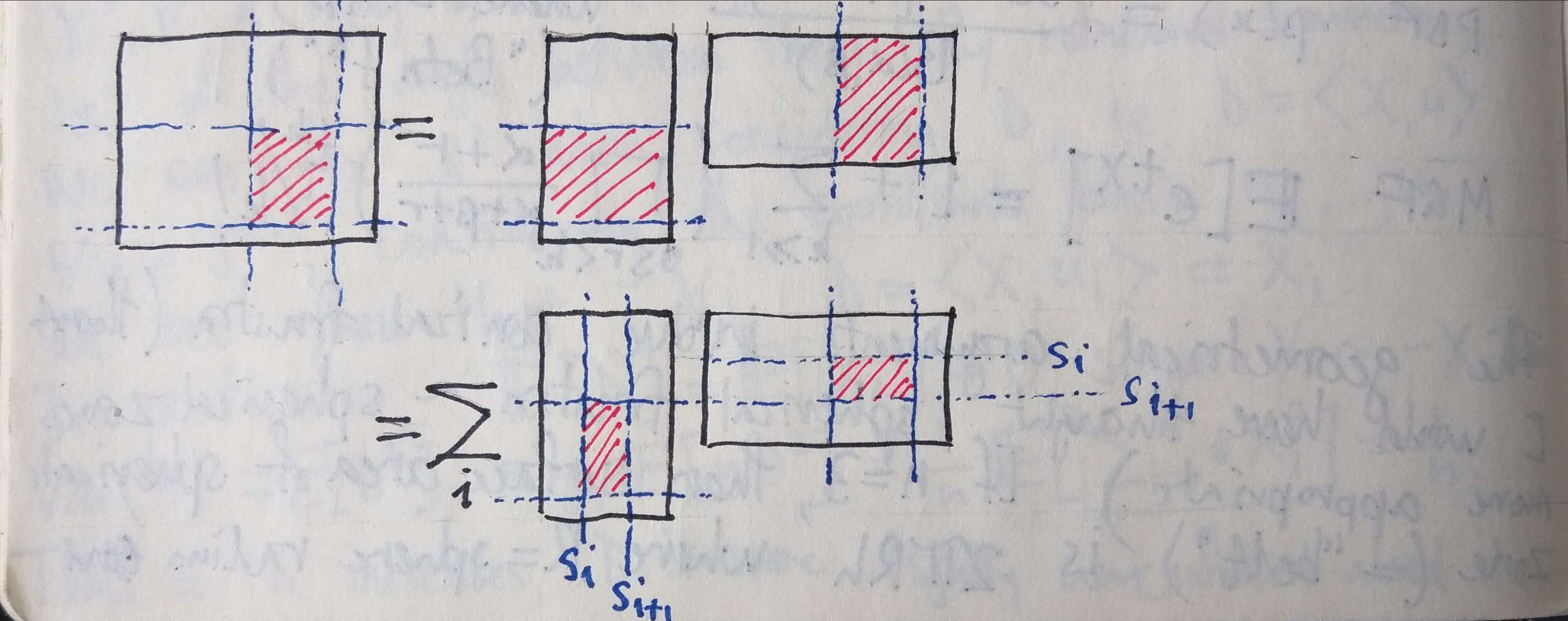
Consider a matrix product . Partition the two outer dimensions (i.e. the rows of and the columns of ) and the one inner dimension (i.e. the columns of and the rows of ) arbitrarily. This defines a “block decomposition” of the product and of the factors such that the blocks of are related to the blocks of and via the familiar formula for components of the product, i.e.
.
Pictorially, we have the following:
Arithmetically, this is easy to prove by considering the formula above for the components of the product. The partitioning of the outer dimensions comes for free, while the partitioning of the inner dimension just corresponds to partitioning the summation:
.
Zooming out to a categorical level, we can see that there is nothing peculiar about this situation. If, in an additive category, we have three objects with biproduct decompositions, and a chain of morphisms:
then this “block decomposition of matrices” finds expression as a formula in using the injection and projection morphisms associated with each biproduct factor.
Below are notes from a talk on Expectation Maximisation I gave at our ML-learning group. Gaussian mixture models are considered as an example application.
Another useful reference is likely the 1977 paper by Dempster et al. that made the technique famous (this is something I would have liked to have read, but didn’t).
Questions
I still don’t understand how EM manages to (reportedly) work so well, given that the maximisation chooses for the next parameter vector precisely the one that reinforces the “fantasy” completions of the data made by the previous parameter vector. I would not have considered it a good learning strategy. It contrasts greatly with, for example, the learning strategy of a restricted Boltzmann machine, in which, at each iteration, the parameters are adjusted so as to correct the model’s fantasy towards producing the observed data.
Can we offer a better argument for why maximisation of the likelihood for latent variable models is difficult?
Is the likelihood of an exponential family distribution convex in the parameters? This is certainly the case for e.g. the mean of a Gaussian. Does this explain why the maximisation of the constructed lower bound for the likelihood is easy?
Here we calculate the entropy of the normal distribution and show that the normal distribution has maximal entropy amongst all distributions with a given finite variance.
The video belong concerns just the calculation of the entropy, not the maximality property.
Shannon makes this claim in his 1948 paper and lists this property as one of his justifications for the definition of entropy. We give a short proof of his claim.
Here we consider the problem of approximately factorising a matrix without constraints and show that solutions can be generated from the orthonormal eigenvectors of the Gram matrix (i.e. of the sample covariance matrix).
(Speculative) can we characterise the solutions as orbits of the orthogonal group on the solutions above, and on those solutions obtained from the above by adding rows of zeros to ?
Under what constraints, if any, are the optimal solutions to matrix factorisation matrices with orthonormal rows/columns? To what extent does orthogonality come for free?
Below is a (rough!) draft of a talk I gave at the Berlin Machine-Learning Learning-Group on the bias-variance trade-off, including the basics of estimator theory, some examples and maximum likelihood estimation.
We show that a real, symmetric matrix has basis of real-valued orthonormal eigenvectors and that the corresponding eigenvalues are real. We show moreover that these eigenvalues are all non-negative if and only if the matrix is positive semi-definite.