zkp – Building Babylon

A polynomial with coefficients in a field and of degree $< n$ is determined by its evaluations at any $n$ distinct points. A common way to see this is via Lagrange interpolation. But what happens in the more general case where the coefficients come from a commutative ring $R$ with $1$ ? It’s easy to see that the statement fails. Consider e.g. $R = Z / 8 Z$ , and let $f (X) = 4 X + 4 X^{2}$ . Then $f$ vanishes everywhere on R (easy to check), despite having degree two. In particular, there are multiple polynomials of degree $< 3$ (viz. $f$ and the zero polynomial) that vanish at three distinct points e.g. $1, 2, 3$ .

The correct generalization of the statement can be derived by considering the Vandermonde matrix. Recall that, given points $c_{1}, \dots, c_{n} \in R$ , the Vandermonde matrix $V$ is the $n$ x $n$ matrix consisting of powers of the $c_{i}$ . The matrix-vector product of $V$ and the vector of the coefficients of a polynomial $f$ then gives the vector of evaluations $f (c_{i})$ of $f$ at the points $c_{i}$ . Interpolation goes the other way, i.e. from evaluations to coefficients. So we’d like to be able to invert the Vandermonde matrix.

As it happens, a square matrix over a commutative ring $R$ with $1$ is invertible if and only if its determinant is invertible in $R$ (the construction of the inverse matrix in terms of the adjugate demonstrates this). The determinant of the Vandermonde can be shown (using only column operations and properties of the determinant) to be the product of the $c_{i} - c_{j}$ for $i \neq j$ . Thus we see that a polynomial $f \in R [X]$ of degree $< n$ is determined by its evaluations at $n$ distinct points if the differences of these evaluation points are invertible in $R$ .

In fact, we can do much better: the differences don’t need to have inverses in $R$ , they just need to be invertible in a larger ring: it in fact suffices that the differences are not zero divisors in $R$ . For suppose that this is the case. Let $S$ be the multiplicative closure of the set of pairwise differences. Then $S$ contains no zero divisors, and so $R$ can be considered as a subring of its localization $S^{- 1} R$ at the subset $S$ . Importantly, the pairwise differences have inverses in $S^{- 1} R$ . Hence, by the above argument, any polynomial of degree $< n$ with coefficients in $S^{- 1} R$ is determined by its evaluations at our points, and this of course continues to hold when the coefficients (and evaluations) lie in the subring $R$ .

To return to the problematic example above: for any three distinct points in $R = Z / 8 Z$ , either at least two of them are odd, or at least two of them are even, and in either case there will be a pair of distinct points whose difference is even and hence either zero or a zero divisor.

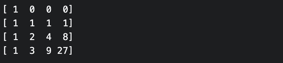
The Vandermonde matrix computes evaluations of polynomials from their coefficients via a matrix-vector product. The Vandermonde matrices are nested, i.e. each Vandermonde matrix is the principal submatrix of any larger Vandermonde matrix that uses (an extension of) the same sequence of evaluation points. For example, here is the (square) Vandermonde matrix for the evaluation points $0, 1, 2, 3$ ; the Vandermonde matrix for $0, 1, 2$ is the $3$ x $3$ principal (i.e. top-left) submatrix:

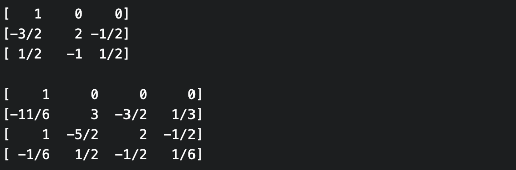
If the inverse Vandermonde matrix exists, then the inverse computation (from evaluations to coefficients, i.e. polynomial interpolation), can also be performed as a matrix-vector product (for the inverse of the Vandermonde matrix to exist, it must be square and the evaluation points must be distinct). Unfortunately, the inverse Vandermonde matrices are no longer “nested” in the above sense. For example, here are the inverse Vandermonde matrices for evaluation points $0, 1, 2$ and $0, 1, 2, 3$ .

Who cares? Well, it would be nice if they were nested since then one could pre-compute a sufficiently large inverse Vandermonde matrix, and be able to interpolate any polynomial that came along. But it just isn’t so! However, for the particular case where the evaluation points are the non-negative integers (and indeed in many more general cases), the neatness can be restored using a certain triangular decomposition of the Vandermonde matrix and its inverse.

Let’s write $V_{n}$ for the Vandermonde matrix for the evaluation points $0, 1, . ., n$ . Then $V_{n}$ can be expressed as a product of an lower-triangular, diagonal and upper-triangular matrices $L_{n}$ , $D_{n}$ , and $U_{n}$ i.e. $V_{n} = L_{n} D_{n} U_{n}$ . Thus $V_{n}^{- 1} = U_{n}^{- 1} D_{n}^{- 1} L_{n}^{- 1}$ . It turns out that all of these factors form nested families in the sense above, e.g. $U_{n}$ is the principal $n$ x $n$ submatrix of any $U_{n + k}$ , while $L_{n}^{- 1}$ is the principal $n$ x $n$ submatrix of $L_{n + k}^{- 1}$ , and so on. Thus if we pre-compute $L_{n}^{- 1}, D_{n}^{- 1}, U_{n}^{- 1}$ then we’ll be able to interpolate any polynomial of degree at most $n$ (by selecting the appropriate principal submatrix of each factor, and then performing three matrix-vector multiplications).

Furthermore, the entries of $L^{- 1}, D^{- 1}, U^{- 1}$ (also of $L$ , $D$ , $U$ ) are given by pleasing and useful recursive formulae, and these can be used to increase the size of your precomputed matrices as required. For instance, $(L^{- 1})_{i, j} = (- 1)^{i - j} (\binom{i}{j})$ and the identity $(\binom{i}{j}) = (\binom{i - 1}{j - 1}) + (\binom{i - 1}{j})$ is easily adapted to a recurrence on the $(L^{- 1})_{i, j}$ that allows us to extend $L^{- 1}$ as needed. The diagonal entries of $D^{- 1}$ are given by $(D^{- 1})_{i, i} = \frac{1}{i!}$ (recurrence obvious) while the entries of $U^{- 1}$ are given by the (signed) Sterling numbers of the first kind via $(U^{- 1})_{i, j} = s (j, i)$ . These quantities satisfy the recurrence $s (j, i) = s (j - 1, i - 1) - (j - 1) s (j - 1, i)$ with boundary conditions $s (0, 0) = 1$ and $s (k, 0) = s (0, k) = 0$ for all $k > 0$ .

These formulae were first derived in Vandermonde matrices on integer nodes (Eisinberg, Franzé, Pugliese; 1998). Another useful (and freely available) reference is Symmetric functions and the Vandermonde matrix (Oruç & Akmaz; 2004) which deals with the case of $q$ -integer nodes (take $q = 0$ in their Theorem 4.1 to obtain the formulae above).

Tag: zkp

When is a polynomial determined by evaluations? Polynomial interpolation over commutative rings with unity.

Efficient polynomial interpolation on $0, 1, 2, . .$ (the inverse Vandermonde on integer nodes)