Graph embeddings in Hyperbolic Space

I gave a talk last night at the Berlin machine learning meetup on learning graph embeddings in hyperbolic space, featuring the recent NIPS 2017 paper of Nickel & Kiela. Covered are:

  • An illustration of why the Euclidean plane is not a good place to embed trees (since circle circumference grows only linearly in the radius);
  • Extending this same argument to higher dimensional Euclidean space;
  • An introduction to the hyperbolic plane and the Poincaré disc model;
  • A discussion of Rik Sarkar’s result that trees embed with arbitrarily small error in the hyperbolic plane;
  • A demonstration that, in the hyperbolic plane, circle circumference is exponential in the radius (better written here);
  • A review of the results of Nickel & Kiela on the (transitive closure of the) WordNet hypernymy graph;
  • Some thoughts on the gradient optimisation (perhaps better written here).

And here are the slides!

Gradient optimisation on the Poincaré disc

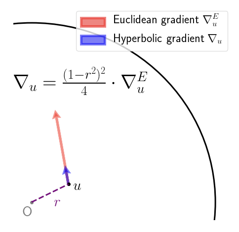
Nickel & Kiela had a great paper on embedding graphs in hyperbolic space at NIPS 2017. They work with the Poincaré ball model of hyperbolic space. This is just the interior of the unit ball, equipped with an appropriate Riemannian metric. This metric is conformal, meaning that the inner product on the tangent spaces on the Poincare ball differ from that of the (Euclidean) ambient space by only a scalar factor. This means that the hyperbolic gradient $\nabla_u$ at a point $u$ can be obtained from the Euclidean gradient $\nabla^E_u$ at that same point just by rescaling. That is, you pretend for a moment that your objective function is defined in Euclidean space, calculate the gradient as usual, and just rescale. This scaling factor depends on the Euclidean distance $r$ of $u$ from the origin, as depicted below:
So far, so good. What the authors then do is simply add the (rescaled) gradient to obtain the new value of the parameter vector, which is fine, if you only take a small step, and so long as you don’t accidentally step over the boundary of the Poincaré disc! A friend described this as the Buzz Lightyear update (“to infinity, and beyond!”). While adding the gradient vector seems to work fine in practice, it does seem rather brutal. The root of the “problem” (if we agree to call it one) is that we aren’t following the geodesics of the manifold – to perform an update, we should really been applying the exponential map at that current point to the gradient vector. Geodesics on the Poincaré disc look like this:
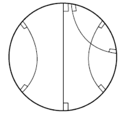
that is, they are sections of circles that intersect the boundary of the Poincaré disc at right angles, or diameters (the latter being a limiting case of the former). With that in mind, here’s a picture showing how the Buzz Lightyear update on the Poincaré disc could be sub-optimal:
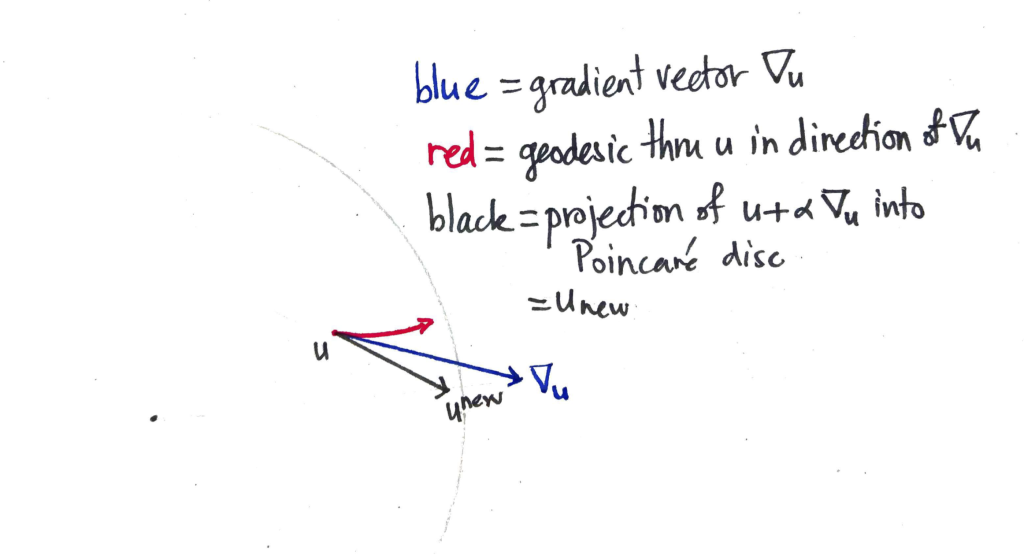
The blue vector $\nabla_u$ is the hyperbolic gradient vector that is added to $u$, taking us out of the Poincaré disc. The resulting vector is then pulled back (along the ray with the faintly-marked origin) until it is within the disc by some small margin, resulting in the new value of the parameter vector $u^\textrm{new}$. On the other hand, if you followed the geodesic from $u$ to which the gradient vector is tangent, you’d end up at the end of the red curve. Which is quite some distance away.

Re-parameterising for non-negativity yields multiplicative updates

Suppose you have a model that depends on real-valued parameters, and that you would like to constrain these parameters to be non-negative. For simplicity, suppose the model has a single parameter $a \in \mathbb R$. Let $E$ denote the error function. To constrain $a$ to be non-negative, parameterise $a$ as the square of a real-valued parameter $\alpha \in \mathbb R$:

$$a = \alpha^2, \quad \alpha \in \mathbb R.$$

We can now minimise $E$ by choosing $\alpha$ without constraints, e.g. by using gradient descent. Let $\lambda > 0$ be the learning rate. We have

\begin{eqnarray*}
\alpha^{\text{new}} &=& \alpha – \lambda \frac{\partial E}{\partial \alpha} \\
&=& \alpha – \lambda \textstyle{\frac{\partial E}{\partial a} \frac{\partial a}{\partial \alpha}} \\
&=& \alpha – \lambda 2 \alpha \textstyle \frac{\partial E}{\partial a} \\
&=& \alpha \cdot (1 – 2 \lambda \textstyle \frac{\partial E}{\partial a})
\end{eqnarray*}

by the chain rule. Thus

\begin{eqnarray*}
a^{\text{new}} &=& (\alpha^{\text{new}})^2 \\
&=& \alpha^2 (1 – 2 \lambda \textstyle\frac{\partial E}{\partial a})^2 \\
&=& a \cdot (1 – 2 \lambda \textstyle\frac{\partial E}{\partial a})^2.
\end{eqnarray*}

Thus we’ve obtained a multiplicative update rule for $a$ that is in terms of $a$, only. In particular, we don’t need $\alpha$ anymore!

Orthogonal transformations and gradient updates

We show that if the contour lines of a function are symmetric with respect to some rotation or reflection, then so is the evolution of gradient descent when minimising that function. Rotation of the space on which the function is evaluated effects a corresponding rotation of each of the points visited under gradient descent (similarly, for reflections).

This ultimately comes down to showing the following: if $ f: \mathbb{R}^N \to \mathbb{R} $ is the differentiable function being minimised and $ g $ is a rotation or reflection that preserves the contours of $ f $, then

\begin{equation}\label{prop} \nabla |_{g(u)} f = g ( \nabla |_u f) \end{equation}

for all points $ u \in \mathbb{R}^N $.

Examples

We consider below three one-dimensional examples that demonstrate that, even if the function $ f $ is symmetric with respect to all orthogonal transformations, it is necessary that the transformation $ g $ be orthogonal in order for the property (\ref{prop}) above to hold.