In a paper with Adriaan Schakel, we presented controlled experiments for word embeddings using pseudo-words. Performing these experiments in the case of word2vec CBOW showed that, in particular, the vector direction of any particular word changed only moderately when the frequency of the word was varied. Shortly before we released the paper, Schnabel et al presented an interesting paper at EMNLP, where (amongst other things), they showed that it was possible to distinguish rare from frequent words using logistic regression on the normalised word vectors, i.e. they showed that vector direction does approximately encode coarse (i.e. binary, rare vs. frequent) frequency information. Here, I wanted to quickly report that the result of Schnabel et al. holds for the vectors obtained from our experiments, as they should. Below, I’ll walk through exactly what I checked.
I took the word vectors that we trained during our experiments. You can check our paper for a detailed account. In brief, we trained a word2vec CBOW model on popular Wikipedia pages with a hidden layer of size 100, negative sampling with 5 negative samples, a window size of 10, a minimum frequency of 128, and 10 passes through the corpus. Sub-sampling was not used so that the influence of word frequency could be more clearly discerned. There were 81k unigrams in the vocabulary. Then:
- the word vectors were normalised so that their (Euclidean-) length was 1.
- the frequency threshold of 5000 was chosen (somewhat arbitrarily) to define the boundary between rare and frequent words. This gave 8428 “frequent” words. A random sample of the same size of the remaining “rare” words was then chosen, so that the two classes, “rare” and “frequent”, were balanced. This yielded approximately 17k data points, where a data point is a normalised word vector labelled with either “frequent” (1) or “rare” (0).
- the data points were split into training- and test- sets, with 70% of the data points in the training set.
- a logistic regression model was fit on the training set. An intercept was fit, but this boosted the performance only slightly. No regularisation was used since the number of training examples wass high compared to the number of parameters.
- The performance on the test set was assessed by calculating the ROC curve on the training and test sets and the accuracy on the test set.
Model performance
Consider the ROC curve below. We see from that fact that the test curve approximately tracks the training curve that the model generalises reasonably to unseen data. We see also from the closeness of the curves to the axes at the beginning and the end that the model is very accurate in detecting frequent words when it gives a high probability (bottom left of the curve) and at detecting infrequent words when it gives a low probability (top right).
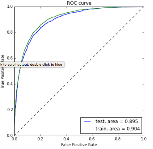
(ROC curve made using a helpful code snippet from sklearn)
The accuracy of the model on the test set was 82%, which agrees very nicely with what was reported in Schnabel et al., summarised in the following image:
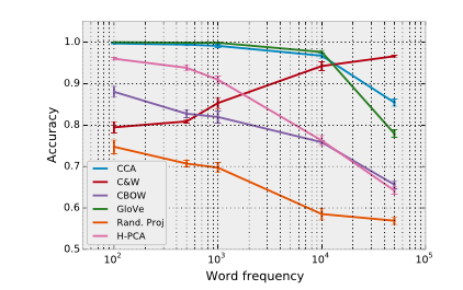
The training corpus and parameters of Schnabel, though not reported in full detail (they had a lot of other things to report), seem similar. We know that their CBOW model was 50 dimensional, had a vocabulary of 103k words, and was trained on the 2008 Wikipedia.