The paper Neural Word Embeddings as Implicit Matrix Factorization of Levy and Goldberg was published in the proceedings of NIPS 2014 (pdf). It claims to demonstrate that Mikolov’s Skipgram model with negative sampling is implicitly factorising the matrix of pointwise mutual information (PMI) of the word/context pairs, shifted by a global constant. Although the paper is interesting and worth reading, it greatly overstates what is actually established, which can be summarised as follows:
Suppose that the dimension of the Skipgram word embedding is at least as large as the vocabulary. Then if the matrices of parameters $(W, C)$ minimise the Skipgram objective, and the rows of $W$ or the columns of $C$ are linearly independent, then the matrix product $WC$ is the PMI matrix shifted by a global constant.
This is a really nice result, but it certainly doesn’t show that Skipgram is performing (even implicitly) matrix factorisation. Rather it shows that the two learning tasks have the same global optimum – and even this is only shown when the dimension is larger than the vocabulary, which is precisely the case where Skipgram is uninteresting.
The linear independence assumption
The authors (perhaps unknowingly) implicitly assume that the word vectors on one of the two layers of the Skipgram model are linearly independent. This is a stronger assumption than what the authors explicitly assume, which is that the dimension of the hidden layer is at least as large as the vocabulary. It is also not a very natural assumption, since Skipgram is interesting to us precisely because it captures word analogies in word vector arithmetic, which are linear dependencies between the word vectors! This is not a deal breaker, however, since these linear dependencies are only ever approximate.
In order to see where the assumption arises, first recall some notation of the paper:
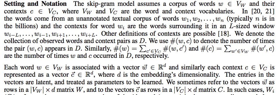
The authors consider the case where the negative samples for Skipgram are drawn from the uniform distribution $P_D$ over the contexts $V_C$, and write

for the log likelihood. The log likelihood is then rewritten as another double summation, in which each summand (as a function of the model parameters) depends only upon the dot product of one word vector with one context vector:
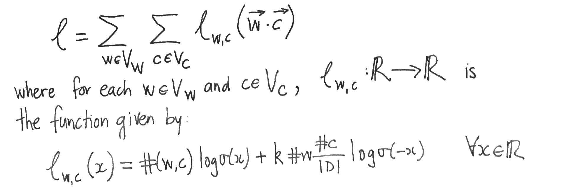
The authors then suppose that the values of the parameters $W, C$ are such that Skipgram is at equilibrium, i.e. that the partial derivatives of $l$ with respect to each word- and content-vector component vanish. They then assume that this implies that the partial derivatives of $l$ with respect to the dot products vanish also. To see that this doesn’t necessarily follow, apply the chain rule to the partial derivatives:

This yields systems of linear equations relating the partial derivatives with respect to the word- and content- vector components (which are zero by supposition) to the partial derivatives with respect to the dot products, which we want to show are zero. But this only follows if one of the two systems of linear equations has a unique solution, which is precisely when its matrix of coefficients (which are just word- or context- vector components) has linearly independent rows or columns. So either the family of word vectors or the family of context vectors must be linearly independent in order for the authors to proceed to their conclusion.
Word vectors that are of dimension the size of the vocabulary and linearly independent sound to me more akin to a one-hot or bag of words representations than to Skipgram word vectors.
Skipgram isn’t Matrix Factorisation (yet)
If Skipgram is matrix factorisation, then it isn’t shown in this paper. What has been shown is that the optima of the two methods coincide when the dimension is larger that the size of the vocabulary. Unfortunately, this tells us nothing about the lower dimensional case where Skipgram is actually interesting. In the lower dimensional case, the argument of the authors can’t be applied, since it is then impossible for the word- or context- vectors to be linearly independent. It is only in the lower dimensional case that the Skipgram and Matrix Factorisation are forced to compress the word co-occurrence information and thereby learn anything at all. This compression is necessarily lossy (since there are insufficient parameters) and there is nothing in the paper to suggest that the two methods will retain the same information (which is what it means to say that the two methods are the same).
Appendix: Comparing the objectives
To compare Skipgram with negative sampling to MF, we might compare the two objective functions. Skipgram maximises the log likelihood $l$ (above). MF, on the other hand, typically minimises the squared error between the matrix and its reconstruction:

The partial derivatives of $E$, needed for a gradient update, are easy to compute:

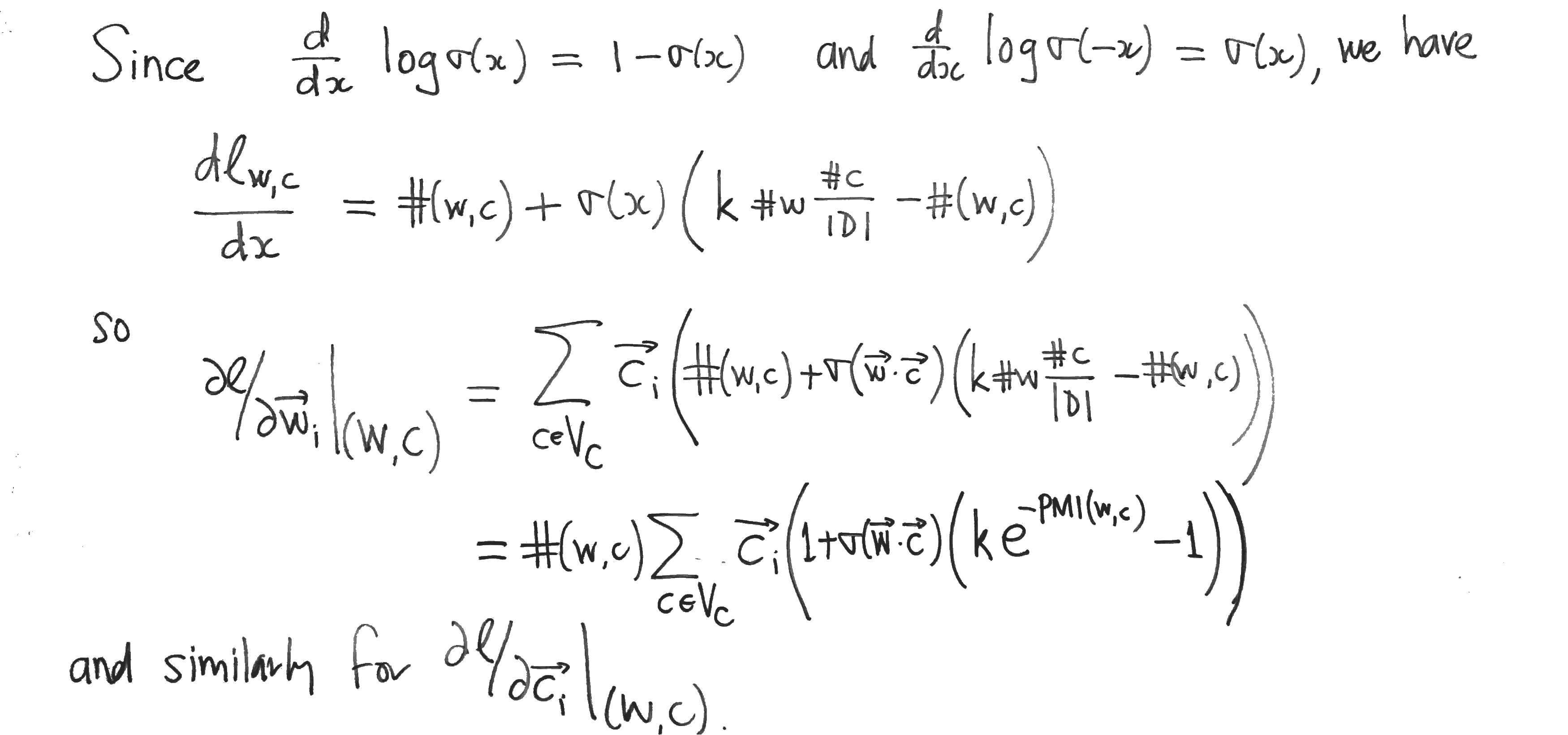
Compare these with the partial derivatives of the Skipgram log-likehood $l$, which can be computed as follows:
