An important step in the soundness analysis of the FRI-IOPP is bounding the probability of an “unlucky fold”: assuming that the prover is cheating (so that the initial oracle is $\delta$-far from the code), how likely is it that the verifier “unluckily” chooses a folding challenge $\alpha \in \ff$ such that the $\alpha$-folding of the oracle is not $\delta$-far from its code? We describe here how to bound this probability using the Correlated Agreement Theorem from [PG-RSC].
Notation
Let $\ff$ be a finite field and suppose $\Omega \subset \ff^\times$ is a multiplicative subgroup with even order, so that $\omega \mapsto \omega^2$ is a 2-to-1 map $\Omega \to \Omega^2$. Write $\ffOmega$ (resp. $\ffOmegaSqrd$) for the space of all $\ff$-valued functions on $\Omega$ (resp. $\Omega^2$). Denote by $\eval_\Omega$ the evaluation map $f \mapsto (f(\omega))_{\omega \in \Omega} \in \ffOmega$, and for any $d > 0$, write $\RSd = \eval_\Omega (\fxd)$ for the Reed-Solomon code consisting of evaluations of polynomials with degree less than $d$ on $\Omega$. Write $\Delta$ for the relative Hamming distance.
Define $\Theta = (\Theta_0, \Theta_1): \ffOmega \to \ffOmegaSqrd \times \ffOmegaSqrd$ by $$ (\Theta_0 u)_{\omega^2} = \frac{u_\omega + u_{-\omega}}{2}, \qquad (\Theta_1 u)_{\omega^2} = \frac{u_\omega – u_{-\omega}}{2\omega}, \qquad \forall \omega \in \Omega,\ \forall u \in \ffOmega.$$ The map $\Theta$, which operates in the evaluation domain, corresponds to the familiar even/odd decomposition of a polynomial in the coefficient domain. In particular: $$u_\omega = (\Theta_0 u)_{\omega^2} + \omega (\Theta_1 u)_{\omega^2}, \qquad \forall \omega \in \Omega,\ \forall u \in \ffOmega,$$ and so the folding $\Psi_\alpha u$ of $u \in \ffOmega$ using $\alpha \in \ff$ can be defined using $\Theta$ via: $$ \Psi_\alpha : \ffOmega \to \ffOmegaSqrd, \qquad u \mapsto (\Theta_0 u) + \alpha (\Theta_1 u), \qquad \forall u \in \ffOmega.$$
The “Correlated Agreement Theorem” $\mathrm{CAT}_{d, \Omega}$
Let $\rho = d/|\Omega|$, and write $\mathrm{CAT}_{d, \Omega}$ for the following statement, proven in [PG-RSC] (as Theorem 4.1): Suppose that $\delta \in (0, \frac{1 – \rho}{2}]$, and that $\uZero, \uOne \in \ffOmega$ are such that $$ |\ \{ \alpha \in \ff \ |\ \Delta (\uZero + \alpha \uOne, \RSd) < \delta \}\ | \geq |\Omega|.$$ Then there exists $\Lambda \subset \Omega$ with $\frac{|\Lambda|}{|\Omega|} \geq 1 – \delta$ and $\fZero, \fOne \in \fxd$ such that $$ \fZero(\lambda) = \uZero_\lambda, \qquad \fOne(\lambda) = \uOne_\lambda, \qquad \forall \lambda \in \Lambda.$$
The Correlated Agreement Theorem & Unlucky Folds
The contrapositive of $\mathrm{CAT}_{d/2, \Omega^2}$ can be used to bound the probability of an unlucky fold as follows.
Assume that $u \in \ffOmega$ is $\delta$-far from $\RSd$. Then $$ \Delta(u, \eval_\Omega f) \geq \delta, \qquad \forall f \in \fxd.$$ Suppose (for contradiction) that there exist $\fZero, \fOne \in \fxdHalf$ and $\Lambda \subset \Omega^2$ with $|\Lambda| / |\Omega^2| \geq 1 – \delta$ and $$ \fZero (\lambda) = (\Theta_0 u)_\lambda, \qquad \fOne (\lambda) = (\Theta_1 u)_\lambda, \qquad \forall \lambda \in \Lambda.$$ Set $f(X) = \fZero(X^2) + \fOne(X^2)$ and write $\sqrt \Lambda = \{ \omega \in \Omega \ | \ \omega^2 \in \Lambda \}$. Then for any $\lambda \in \Lambda$ and either of its two square roots $\omega \in \sqrt \Lambda$: $$ f(\omega) = \fZero(\lambda) + \omega \fOne(\lambda) = (\Theta_0 u)_\lambda + \omega (\Theta_1 u)_\lambda = u_\omega,$$ and so $f \in \fxd$ and $u \in \ffOmega$ agree on a subset $\sqrt \Lambda \subset \Omega$ of density $$ \frac{|\sqrt \Lambda|}{|\Omega|} = \frac{|\Lambda|}{|\Omega^2|} \geq 1 – \delta.$$ Thus we would have that $\Delta(u, \eval_\Omega f) < \delta$, which would contradict the $\delta$-farness of $u$ from the code. Thus no such $\fZero$, $\fOne$ and $\Lambda$ exist. Therefore, by the contrapositive of $\mathrm{CAT}_{d/2, \Omega^2}$, we have that $$ |\ \{ \ \alpha \in \ff \ |\ \Delta (\Theta_0u + \alpha \Theta_1 u, \RSdHalf) < \delta \ \}\ | < |\Omega|.$$ i.e. that the probability of the folding $\Psi_\alpha u$ failing to be $\delta$-far from $\RSdHalf$ (an “unlucky fold”) is strictly less than $\epsilon = \frac{|\Omega|}{|\ff|}$.
Proving the Correlated Agreement Theorem
The Correlated Agreement Theorem, in the case where $\delta$ is at most the unique decoding radius, can be proven by running the Berlekamp-Welch decoder over the function field $\ff (\alpha)$ (where $\alpha$, transcendental over $\ff$, stands in for the folding challenge). This works since the Berlekamp-Welch decoder is really just a result from linear algebra, and so works over any field. The other ingredient is the Polishchuk-Spielman Lemma. A proof of the theorem and this lemma are given in [PG-RSC].
References
[PG-RSC]: E. Ben-Sasson, D. Carmon, Y. Ishai, S. Kopparty and S. Saraf, “Proximity Gaps for Reed–Solomon Codes,”, 2020 (pdf).
“How to Prove False Statements: Practical Attacks on Fiat-Shamir” (Khovratovich, Rothblum, Soukhanov; 2025) constructs families of circuits for which the GKR protocol, when made non-interactive by Fiat-Shamir heuristic, will prove false statements. It’s a great paper and is so well written that I won’t attempt to do better by paraphrasing their constructions. What I’d like to look at here is instead the consequences of the result for real-world applications of non-interactive proofs.
The Fiat-Shamir heuristic attempts to simulate, in the non-interactive setting, random challenges that the verifier would have issued in an interactive setting. It does so by replacing the information-theoretic assumption of the random oracle model with a cryptographic assumption about deterministic hash functions. Fiat-Shamir is crucial to real-world cryptographic applications (and blockchains, in particular) because it enables non-interactive proofs: a non-interactive proof can be checked by any number of verifiers, present and future. Moreover these verifiers don’t need to trust one another. They can check the validity of the proof for themselves.
How does Fiat-Shamir work? The prover (and any future verifiers), replace each random message from the verifier with the result of applying a cryptographic hash function to all of the messages from the prover up to that point. Intuitively, the cryptographic assumptions on the hash function should then prevent a computationally-bounded malicious prover from choosing their messages to obtain a desired (Fiat-Shamir generated) message from the verifier and thereby prove a false statement. This has never been proven, however, and indeed earlier work had demonstrated somewhat contrived protocols where it fails.
The current paper shows that the Fiat-Shamir heuristic fails for the very natural and useful GKR protocol. In my assessment, this paper is very impactful in a social sense, in that it reminds us all of the fallibility of cryptographic conjectures. It is a blow to the confidence of those building blockchain applications, and also to those who use blockchains as a store of wealth. However, this is not because this specific attack can be carried out in meaningful applications, but simply because it reminds us how we tend to build castles on sand. Moreover, the result “breaks the promise” of GKR in that it illustrates how GKR can, for certain maliciously constructed circuits, prove false statements. Importantly, however, the paper demonstrates failure of non-interactive GKR only for a contrived family of circuits, and so there is a strong sense in which this result has no practical consequences whatsoever. A verifying party is not simply checking “is this a valid proof of the satisfaction of some circuit?” but rather “is this a valid proof of satisfaction of the circuit XYZ known to me”. Any verifying party that doesn’t care which circuit is satisfied before it releases the funds (or performs some critical function) was already vulnerable to deception, irrespective of this result. Why would you trust a circuit that you hadn’t audited?
It has also been suggested that this paper signals the end of recursive verification of GKR circuits. The reason for this being that both this attack and recursive verification rely on being able to circuitize the hash function used in the transcript, and so facilitating one facilitates the other. This concern evaporates however when we again remember that the only circuits used in production are ones upon which the prover and verifying parties have agreed, and this includes circuits for recursive verification. Why would a verifying party accept the use of a recursive verifier circuit with a backdoor in it? They simply wouldn’t.
$\newcommand{\fxd}[0]{\mathbb{F}[X]^{< d}} \newcommand{\fxdone}[0]{\mathbb{F}[X]^{< d-1}} \newcommand{\RS}[0]{\mathrm{RS}} \newcommand{\drc}[0]{\mathrm{D}_{r, c}\,} \newcommand{\fo}[0]{\ff^\Omega} \newcommand{\eval}[0]{\mathrm{E}}$ Here we cover how to build a polynomial commitment scheme (PCS) from the FRI interactive oracle proof of proximity (FRI-IOPP). Specifically, we explain how to reduce an evaluation proof to a proof of proximity. It is assumed that the reader already understands the FRI-IOPP. Everything here was derived from reading Transparent PCS with polylogarithmic communication complexity (Vlasov & Panarin, 2019), along with (to be honest) much reflection and discussion.
We assume the usual setup for FRI. Let $\ff$ denote a finite field, write $\Omega \subset \ff$ for a subgroup of the group of units $\ff^\times$ with $|\Omega|$ a power of two. Let $\fo$ denote the vector space of functions $\Omega \to \ff$, considered as vectors with entries indexed by some fixed enumeration of $\Omega$ (we’ll call elements of $\fo$ “words”). Let $\eval: \fx \to \fo$ denote the evaluation map, i.e. $$ (\eval f)_\omega = f(\omega) \quad \forall f \in \fx \quad \forall \omega \in \Omega.$$ Write $\Delta$ for the relative Hamming distance on $\fo$, and let $\RS_k = \eval (\fx^{< k}) \subset \fo$ denote the Reed-Solomon code with degree bound $k$. Fix throughout some degree bound $1 < d < |\Omega|$. We will be concerned with two separate Reed-Solomon codes, namely $\RS_d$ and $\RS_{d-1}$ (note that both use the same evaluation points $\Omega$). Write $\delta_0$ for the unique decoding radius of $\RS_d$, i.e. $\delta_0$ is maximal such that, for any $f \in \fxd$ and $u \in \fo$, $$ \Delta(u, \eval f) \leqslant \delta_0 \implies \left( \ \forall g \in \fxd \quad \Delta(u, \eval g) \leqslant \delta_0 \implies f = g \ \right).$$
The data of a commitment in the FRI-PCS with degree bound $d$ is a word $u \in \fo$ (more precisely: an oracle to $u$). Assume for now that the prover is honest. In the simplest case, $u = \eval f$ for some $f \in \fxd$. Crucially, however, we require something weaker than this of a commitment $u$: it is sufficient that $u$ be within the unique decoding radius of some codeword $\eval f$, i.e. $$\begin{equation}\label{UDR}\tag{UDR} \Delta (u, \eval f) \leqslant \delta_0 \quad \exists f \in \fxd.\end{equation}$$ Any such $u$ is considered to be a valid commitment to its corresponding $f \in \fxd$. Why is this subtlety necessary? Because if the stricter condition $u = \eval f$ were required, then the (soon to be explained) reduction of an evaluation proof to an invocation of the FRI-IOPP wouldn’t be possible. The FRI-IOPP isn’t sufficiently sensitive to reliably distinguish between a codeword and nearby non-codewords (for an explicit demonstration, see here).
Assuming that the prover has sent a commitment $u \in \fo$ to the verifier, an evaluation proof proceeds as follows. The verifier chooses an evaluation point $r \in \ff \setminus \Omega$ and sends this to the prover, and the prover responds with the purported evaluation $c$ of the polynomial committed to (in the case of an honest prover, $c = f(r)$ where $f$ is determined by \eqref{UDR}). The prover wants to establish $$\begin{equation}\label{TwoPart}\tag{TwoPart} \exists f \in \fxd \quad \st \quad \Delta(u, \eval f) \leqslant \delta_0 \ \ \text{and} \ \ f(r) = c.\end{equation}$$ Since $f(r) = c$ if and only if $f-c$ is divisible by $X-r$, and degree is additive under polynomial multiplication, this two part claim is equivalent to the following unified claim: $$\begin{equation}\label{Unified}\tag{Unified} \exists q \in \fxdone \quad \st \quad \Delta(u, \eval ((X-r)q + c)) \leqslant \delta_0.\end{equation}$$ Thus we are interested in the proximity of the commitment $u$ to a specific subset of $\RS_d$, namely the subset consisting of codewords of the form $\eval ((X-r)q + c)$. Note, however, that we can not immediately apply FRI-IOPP to establish this claim, since this subset is not itself a Reed-Solomon code (it isn’t even a linear subspace of $\fo$). The good news is that, with a small amount of work, it can be seen that the claim \eqref{Unified} is equivalent to a claim that can be established using the FRI-IOPP (with degree bound $d-1$). This claim involves a vector $\drc u \in \fo$ derived from $u$, which we’ll define below. And thus the FRI-PCS evaluation proof will be established using by a proximity proof!
Firstly, a note on oracles. Importantly, the verifier does not need to receive or read all of the $u \in \fo$ that commits to $f \in \fxd$. Since an evaluation proof reduces to an invocation of the FRI-IOPP, it is sufficient for the verifier to be supplied with a mechanism to query entries $u_\omega$ of $u$ at arbitrary indices $\omega \in \Omega$. In an information theoretic presentation, this mechanism is abstracted as an oracle. In implementation, the oracle is typically instantiated with a Merkle commitment to the tree whose leaves are the $u_\omega$ (enumerated in some agreed upon manner). The prover binds itself to $u$ by sending the Merkle root to the verifier, and the verifier queries an entry $u_\omega$ by asking the prover for the Merkle path from the root to the corresponding leaf.
Let’s now derive the reduction of the evaluation proof to an instance of the FRI-IOPP. Given bijections $\theta_w : \ff \to \ff$ for each $\omega \in \Omega$, a bijection $\theta : \fo \to \fo$ of the space of all words can be defined by $$(\theta v)_\omega = \theta_\omega (v_\omega) \quad \forall v \in \fo,\quad \forall \omega \in \Omega.$$ Call such a map $\theta$ a “component-wise bijection”; it is immediate for any such map that $$\begin{equation}\label{HDInv}\tag{HDInv} \Delta(\theta u,\ v) = \Delta(u,\ \theta^{-1} v) \quad \forall u, v \in \fo.\end{equation}$$ For any $r \in \ff \setminus \Omega$ and $c \in \ff$, define a component-wise bijection $\drc: \fo \to \fo$ by $$ (\drc u)_\omega = \frac{u_\omega – c}{\omega – r} \quad \forall u \in \fo, \quad \forall \omega \in \Omega.$$ Its inverse is given by $$ (\drc^{-1} (v))_\omega = (\omega – r) v_\omega + c \quad \forall v \in \fo, \quad \forall \omega \in \Omega,$$ from which it follows immediately that $$\begin{equation}\label{DrcInverse}\tag{DrcInverse} (\drc^{-1} \circ \eval) (q) = \eval ( (X-r) q + c) \quad \forall q \in \fx.\end{equation}$$ Combining \eqref{HDInv} and \eqref{DrcInverse}, we obtain $$\begin{equation}\label{StepDown}\tag{StepDown} \Delta(\drc u,\ \eval (q)) = \Delta(u,\ \eval((X-r)q + c)) \quad \forall v \in \fo \quad \forall q \in \fx,\end{equation}$$ and substituting this into the claim \eqref{Unified}, we obtain the equivalent claim $$\begin{equation}\label{FRIable}\tag{FRIable} \exists q \in \fxdone \quad \st \quad \Delta(\drc u, \eval q) \leqslant \delta_0,\end{equation}$$ which the prover and verifier can establish using the FRI-IOPP! \eqref{FRIable} is nothing more than the statement that $\drc u$ is $\delta_0$-close to $\RS_{d-1}$.
Cheating fails (w.h.p.)
It is instructive to now consider the two possible cheating strategies for the prover in this reduction to the FRI-IOPP. The first is where the first claim of \eqref{TwoPart} doesn’t hold, i.e. for all $f \in \fxd$, $u$ is not within the unique decoding radius of some $\eval f$. Put differently, this is just saying that $\Delta(u,\ \RS_d) > \delta_0$, i.e. “$u$ is $\delta_0$-far from the code $\RS_d$”. Thus, by \eqref{StepDown}, for any $q \in \fxdone$, $$ \Delta(\drc u,\ \eval q) = \Delta(u,\ \eval ((X-r)q + c)) \geqslant \Delta(u,\ \RS_d) > \delta_0,$$ and so claim \eqref{FRIable} is false, and will be caught with the soundness bound of the FRI-IOPP. The only other cheating strategy for the prover is that where the $u$ is in the unique decoding radius of $\eval f$ for some $f \in \fxd$, but the claimed evaluation is false, i.e. $f(r) \ne c$. Then for any $q \in \fxdone$, we have $f \ne (X-r)q + c$ (since otherwise the evaluations at $c$ would match), and so $\eval f$ and $\eval ((X-r)q + c)$ are distinct codewords. Thus, by \eqref{StepDown}, $$\Delta(\drc u,\ \eval q) = \Delta(u,\ \eval ((X-r) q + c)) > \delta_0,$$ since $u$ can be within $\delta_0$ (the unique decoding radius) of at most one codeword (which is $\eval f$).
How to perform the FRI-IOPP with degree $d-1$?
The FRI-IOPP is defined for degree bounds $d$ that are powers of two. But if $d$ is a power of two, how to perform the second FRI-IOPP, which uses the degree bound $d-1$? The short answer is simply to replace it with another invocation of the FRI-IOPP with degree bound $d$. In detail:
The verifier will use the oracle to $u$ to simulate an oracle $\drc u$ to $(f-c)/(X-r)$.
The prover wishes to establish that $\drc u$ is within the unique decoding radius (UDR) of $\RS_{d-1}$. The UDR for $\RS_{d-1}$ is larger than the UDR $\delta_0$ for $\RS_d$, so it is sufficient to show that $\Delta(\drc u,\ \RS_{d-1}) < \delta_0$.
Prover and verifier use the FRI-IOPP to instead show that $\Delta(\drc u,\ \RS_d) < \delta_0$. This shows that there exists some $q \in \fxd$ such that $\Delta(\drc u,\ \eval q) < \delta_0$.
By equation \eqref{StepDown}, it follows that $\Delta(u,\ (X-r)q + c) < \delta_0$.
But we are within the UDR, so $(X-r)q + c = f$, where $f$ is the polynomial from the first IOPP invocation. Thus $\text{deg}(q) = \text{deg} (f) – 1$. The first FRI-IOPP showed that $\text{deg} (f) < d$, and so $\eval q \in \RS_{d-1}$. Thus \eqref{Unified} is established, and we are done.
(The following thought experiment was suggested to me by my colleague Ryan Cao; mistakes and invective are my own).
FRI is often described as a “low degree test”, which suggests that the verifier should reject with high probability if the degree is high. This is not the case, as the simple example below demonstrates. Indeed it is the polynomials of highest degree that have the highest chance of being erroneously accepted by the verifier. (What is true is that the FRI verifier rejects with high probability if the evaluations are far from the code: FRI is a proof of proximity).
Let $\mathbb{F}$ be a field, $\Omega \subset \mathbb{F}$ with $n = |\Omega|$, and write $$ \epsilon_\Omega : \mathbb{F}[x]^{<n} \to \mathbb{F}^\Omega, \qquad f \mapsto (f(\omega))_{\omega \in \Omega} $$ for the evaluation map. For any $k \leq n$, let $\text{RS}[\Omega, k] := \epsilon_\Omega (\mathbb{F}[x]^{< k})$ be the Reed-Solomon code of evaluations of polynomials of degree strictly less than $k$ on $\Omega$.
Henceforth we assume that $\Omega$ is a subgroup of the multiplicative group $\mathbb{F}^\times$ and that $n = |\Omega|$ is a power of two. The degree bound $k=2^d$ will also be a power of two. For $\alpha \in \mathbb{F}$, let $\Phi_\alpha : \mathbb{F}[x] \to \mathbb{F}[x]$ be the FRI folding operation (in the coefficient domain) and write $\Psi_\alpha = \epsilon_\Omega \circ \Phi_\alpha \circ \epsilon_\Omega^{-1}$ for the corresponding operation in the evaluation domain. Then it’s not hard to check that for any $v \in \mathbb{F}^\Omega$ and $\alpha \in \mathbb{F}$, we have $$\begin{equation}\textstyle \tag{Fold}\label{Fold} (\Psi_\alpha(v))_{\omega^2} = \frac{1}{2} (1 + \frac{\alpha}{\omega}) v_{\omega} + \frac{1}{2} (1 – \frac{\alpha}{\omega}) v_{-\omega} \quad \forall \omega \in \Omega.\end{equation}$$
FRI operates by iterated folding, using challenges provided by the verifier. The claim of the proximity of $v^{(0)} := v \in \mathbb{F}^\Omega$ to the code $\text{RS}[\Omega, 2^d]$ is reduced to the claim of the proximity of $v^{(1)} := \Psi_\alpha v^{(0)}$ to the code $\text{RS}[\Omega^2, 2^{d-1}]$ for some $\alpha \in \mathbb{F}$. This process is repeated until the claim is that $v^{(d)}$ is close to the code $\text{RS}[\Omega^{2^d}, 1]$, at which point the verifier queries $t$ entries from $v^{(d)}$ and checks if they all agree: if they do, it concludes that $v^{(d)}$ is (w.h.p.) close to its code, and hence that the original vector $v^{(0)}$ is (w.h.p.) close to the original code. Proving that FRI is indeed a good test of proximity is complicated. It is easy to show, however, that FRI is not (indeed never intended being) a reliable means of detecting polynomials of high degree, and that is what we’ll do here.
For any $\omega \in \Omega$, let $L_{\omega, \Omega}$ denote the Lagrange interpolation polynomial, i.e. $$ L_{\omega, \Omega} = \prod_{\substack{\omega’ \in \Omega \ \omega’ \neq \omega}} \frac{x – \omega’}{\omega – \omega’} \in \mathbb{F}[x].$$ Then $\text{deg} L = n – 1$, i.e. it has has maximal degree (given the size of the evaluation domain $\Omega$). Its evaluations, however, are “one-hot” at $\omega$ $$ v_{\omega, \Omega} := \epsilon_\Omega (L_{\omega, \Omega}) = (0, \dots, 0, 1, 0, \dots, 0) $$ and in this sense are maximally close to the code, while not being in the code (having Hamming distance $1$ from the zero codeword). It’s easy to see from \eqref{Fold} that $$ \Psi_\alpha(v_{\omega, \Omega}) = \frac{1}{2} (1 + \frac{\alpha}{\omega}) v_{\omega^2, \Omega^2} $$ i.e. that except with negligible probability (when $\alpha=-\omega$), the folding will also have Hamming distance 1 from its code $\text{RS}[\Omega^2, 2^{d-1}]$. Note, however, that the relative Hamming distance has doubled, since the size of the evaluation domain has halved.
So let’s set $v^{(0)} := v_{\omega, \Omega}$. Then after $d$ rounds of folding, $v^{(d)}$ is (except with negligible probability) non-zero in exactly one place, and its relative distance from the code $\text{RS}[\Omega^{2^d}, 1]$ (which consists of constant vectors) is $2^d / 2^n$ i.e. the rate $\rho$ of the original code. The verifier thus accepts with probability $(1 – \rho)^t$. Given that $\rho$ is typically close to zero (e.g. $2^{22-64}$) and $t$ is always small, this probability is close to $1$. For this reason, it is misleading (if commonplace) to describe FRI as a “low-degree test”: the polynomials $L_{\omega, \Omega}$, which have maximal degree are routinely accepted by the FRI verifier. Why? Because the evaluations of these polynomials are close (“proximal”) to the code. FRI is a proof of proximity, after all.
A polynomial with coefficients in a field and of degree $< n$ is determined by its evaluations at any $n$ distinct points. A common way to see this is via Lagrange interpolation. But what happens in the more general case where the coefficients come from a commutative ring $R$ with $1$? It’s easy to see that the statement fails. Consider e.g. $R = \mathbb{Z}/ 8\mathbb{Z}$, and let $f(X) = 4X + 4X^2$. Then $f$ vanishes everywhere on R (easy to check), despite having degree two. In particular, there are multiple polynomials of degree $< 3$ (viz. $f$ and the zero polynomial) that vanish at three distinct points e.g. $1, 2, 3$.
The circumstances under which a polynomial over a commutative ring is determined by its evaluations can be determined by considering the Vandermonde matrix. Recall that, given points $c_1, \dots, c_n \in R$, the Vandermonde matrix $V$ is the $n$ x $n$ matrix consisting of powers of the $c_i$. The matrix-vector product of $V$ and the vector of the coefficients of a polynomial $f$ then gives the vector of evaluations $f(c_i)$ of $f$ at the points $c_i$. Interpolation goes the other way, i.e. from evaluations to coefficients. So we’d like to be able to invert the Vandermonde matrix.
As it happens, a square matrix over a commutative ring $R$ with $1$ is invertible if and only if its determinant is invertible in $R$ (the construction of the inverse matrix in terms of the adjugate demonstrates this). The determinant of the Vandermonde can be shown (using only column operations and properties of the determinant) to be the product of the differences $c_i – c_j$ for $i \ne j$. Thus we see that a polynomial $f \in R[X]$ of degree $< n$ is determined by its evaluations at $n$ distinct points if the differences of these evaluation points are invertible in $R$.
In fact, we can do much better: the differences don’t need to have inverses in $R$, they just need to be invertible in a larger ring: it in fact suffices that the differences are not zero divisors in $R$. For suppose that this is the case. Let $S$ be the multiplicative closure of the set of pairwise differences. Then $S$ contains no zero divisors, and so $R$ can be considered as a subring of its localization $S^{-1}R$ at the subset $S$. Importantly, the pairwise differences have inverses in $S^{-1}R$. Hence, by the above argument, any polynomial of degree $< n$ with coefficients in $S^{-1}R$ is determined by its evaluations at our points, and this of course continues to hold when the coefficients (and evaluations) lie in the subring $R$.
To return to the problematic example above: for any three distinct points in $R = \mathbb{Z}/ 8\mathbb{Z}$, either at least two of them are odd, or at least two of them are even, and in either case there will be a pair of distinct points whose difference is even and hence either zero or a zero divisor.
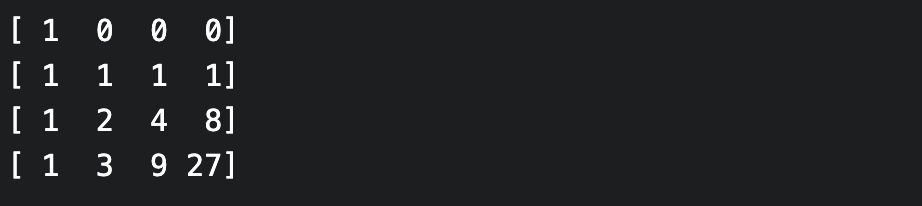
The Vandermonde matrix computes evaluations of polynomials from their coefficients via a matrix-vector product. The Vandermonde matrices are nested, i.e. each Vandermonde matrix is the principal submatrix of any larger Vandermonde matrix that uses (an extension of) the same sequence of evaluation points. For example, here is the (square) Vandermonde matrix for the evaluation points $0, 1, 2, 3$; the Vandermonde matrix for $0, 1, 2$ is the $3$ x $3$ principal (i.e. top-left) submatrix:
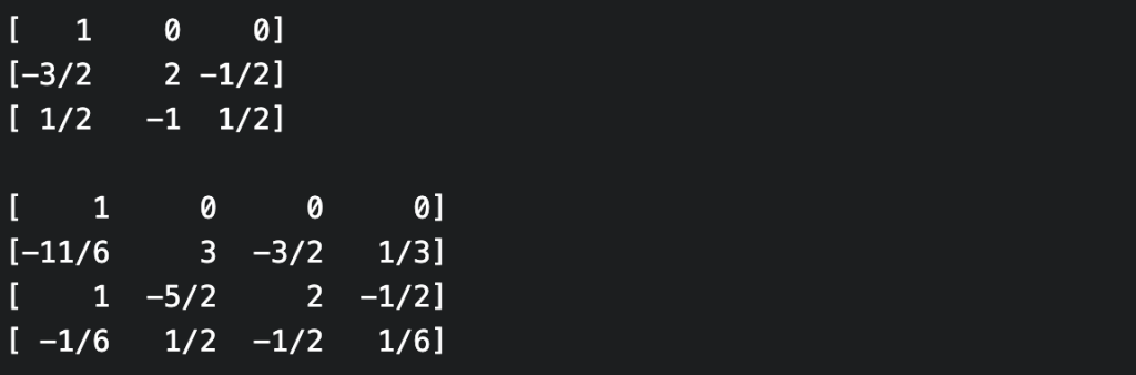
If the inverse Vandermonde matrix exists, then the inverse computation (from evaluations to coefficients, i.e. polynomial interpolation), can also be performed as a matrix-vector product (for the inverse of the Vandermonde matrix to exist, it must be square and the evaluation points must be distinct). Unfortunately, the inverse Vandermonde matrices are no longer “nested” in the above sense. For example, here are the inverse Vandermonde matrices for evaluation points $0, 1, 2$ and $0, 1, 2, 3$.
Who cares? Well, it would be nice if they were nested since then one could pre-compute a sufficiently large inverse Vandermonde matrix, and be able to interpolate any polynomial that came along. But it just isn’t so! However, for the particular case where the evaluation points are the non-negative integers (and indeed in many more general cases), the neatness can be restored using a certain triangular decomposition of the Vandermonde matrix and its inverse.
Let’s write $V_n$ for the Vandermonde matrix defined by the evaluation points $0, 1, .., n$. Then $V_n$ can be expressed as a product of a lower-triangular, diagonal and upper-triangular matrices $L_n$, $D_n$, and $U_n$ i.e. $V_n = L_n D_n U_n$. Thus $V_n^{-1} = U_n^{-1} D_n^{-1} L_n^{-1}$. It turns out that all of these factors form nested families in the sense above. For example, $U_n$ is the principal $n$ x $n$ submatrix of any $U_{n+k}$, while $L_n^{-1}$ is the principal $n$ x $n$ submatrix of $L_{n+k}^{-1}$, and so on. Thus if we pre-compute $L_n^{-1}, D_n^{-1}, U_n^{-1}$ then we’ll be able to interpolate any polynomial of degree at most $n$ (by selecting the appropriate principal submatrix of each factor, and then performing three matrix-vector multiplications).
Furthermore, the entries of $L^{-1}, D^{-1}, U^{-1}$ (also of $L$, $D$, $U$) are given by pleasing and useful recursive formulae, and these can be used to increase the size of your precomputed matrices as required. For instance, $(L^{-1})_{i,j} = (-1)^{i-j} \binom{i}{j}$ and the identity $$\binom{i}{j} = \binom{i-1}{j-1} + \binom{i-1}{j}$$ is easily adapted to a recurrence on the $(L^{-1})_{i,j}$ that allows us to extend $L^{-1}$ as needed. The diagonal entries of $D^{-1}$ are given by $(D^{-1})_{i,i} = \frac{1}{i!}$ (recurrence obvious) while the entries of $U^{-1}$ are given by the (signed) Sterling numbers of the first kind via $(U^{-1})_{i,j} = s(j,i)$. These quantities satisfy the recurrence $$s(j, i) = s(j-1, i-1) – (j-1) s(j-1,i)$$ with boundary conditions $s(0,0) = 1$ and $s(k, 0) = s(0, k) = 0$ for all $k > 0$.
These formulae were first derived in Vandermonde matrices on integer nodes (Eisinberg, Franzé, Pugliese; 1998). Another useful (and freely available) reference is Symmetric functions and the Vandermonde matrix (Oruç & Akmaz; 2004) which deals with the case of $q$-integer nodes (take $q=0$ in their Theorem 4.1 to obtain the formulae above).
The following is intended as an introduction to finite fields for those with already some familiarity with algebraic constructions. It is based on a talk given at our local seminar.
A finite field is simply a field with a finite number of elements. An example of a finite field that should already be familiar is $\mathbb{Z} / p \mathbb{Z}$, the integers modulo a prime $p$, which in the context of field theory is more commonly denoted $\mathbb{F}_p$. But what other finite fields exist? In this post, we’ll construct a finite field $\mathbb{F}_{p^n} = GF(p^n)$ of size $p^n$ for any prime $p$ and positive integer $n$, and additionally prove that, up to isomorphism, these are all the finite fields.
(Note that another common notation for $\mathbb{F}_{p^n}$ is $GF(p^n)$ – the “GF” stands for “Galois field”).
$\mathbb{F}_p$ is a field
Firstly, let’s take a moment to show why $\mathbb{F}_p$ is a field. It is clearly is a commutative ring with 1, so it remains to see why every non-zero element $a$ has an inverse. We need to find an element $x$ such that $ax \equiv 1 \mod p$. The Extended Euclidean Algorithm provides a way to find such a $x$. The algorithm takes two positive integers $a, b$ and returns integer coefficients that linearly combine $a$ and $b$ to yield their GCD, i.e. such that $ax + by = \gcd(a, b)$. Take $b=p$. Since $p$ is prime and $a$ is not zero, $\gcd(a, p) = 1$. The Euclidean algorithm therefore yields $x$ and $y$ such that $ax + py = 1$, which means $ax \equiv 1 \mod p$. Hence, $x$ is the multiplicative inverse of $a$.
This same argument will be recycled below in our construction of extension fields.
The characteristic of a field
The characteristic of a field $K$ is the smallest positive integer $p$ such that $p \cdot 1 := 1 + \cdots + 1$ ($p$ times) equals $0$ in $K$. In other words, it is the order of the additive group generated by the element $1$.
If $K$ is finite, then it is clear that such a $p$ must exist. Moreover, $p$ must be prime. For supposing that $p$ factorized, as say $p=rs$ with $1 < r, s < p$, it would follow that \begin{equation}\label{ZD}\tag{ZD}(r \cdot 1) (s \cdot 1) = 0,\end{equation} while at the same time, by minimality of the characteristic, we’d have that neither of the multiplicands $r\cdot 1$, $s \cdot 1$ were themselves zero. To arrive at a contradiction, either note that you’ve constructed zero divisors in a field, or instead use that fact that $r \cdot 1$ (being non-zero) has an inverse, multiply both sides of \eqref{ZD} by that inverse and note that this would force $s \cdot 1 = 0$, a contradiction.
(A similar argument shows that $\mathbb{Z} / m\mathbb{Z}$ is not a field if $m$ is not prime).
If no positive integer $p$ exists such that $p \cdot 1 = 0$, the characteristic is defined to be zero (this is the case for $\mathbb{Q}, \mathbb{R}, \mathbb{C}$, for example).
The prime subfield
A subfield of a field is simply a subset which is itself a field (with the same $1$ and $0$). The prime subfield of a field $K$ is the subfield generated by $1$ and is the smallest subfield contained in $K$. If the characteristic of $K$ is a prime number $p$, then the prime subfield is (a copy of) the field $\mathbb{F}_p$. If the characteristic of $K$ is zero, then the prime subfield is isomorphic to the field of rational numbers $\mathbb{Q}$.
Of course, the prime subfield could be the entire field!
Any finite field has size a prime power, and that prime is its characteristic
Let $K$ be a finite field of characteristic $p$, and identify $\mathbb{F}_p$ with the prime subfield of $K$. Now let’s forget some of the structure of $K$ and just consider $K$ as a vector space over the field $\mathbb{F}_p$. The vector space axioms are indeed satisfied, since elements of $K$ can be added together, and multiplied by scalars (i.e. elements of $\mathbb{F}_p$) in a way that is distributive and associative – all of this just follows from the field axioms.
Now let $n \geq 1 $ be the dimension of $K$ as a vector space over $\mathbb{F}_p$. If you chose a basis for $K$, it would have length $n$, and every element of $K$ would have a unique expression as a linear combination of the basis with coefficients in $\mathbb{F}_p$. Moreover, every such expression would be an element of $K$. There are $p^n$ such expressions, so $| K | = p^n$.
Example: there is precisely one field with four elements
While we will indeed construct $\mathbb{F}_{p^n}$ for every prime $p$ and $n >0$, let’s first do the simplest possible example beyond the more familiar fields $\mathbb{F}_p$: let’s “manually” construct a field $\mathbb{F}_4$ with four elements. Indeed, we’ll see that there is only one such field, up to isomorphism.
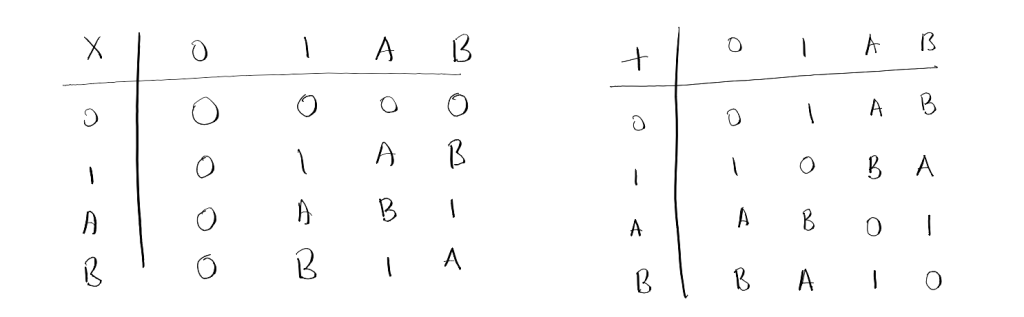
Firstly, note that $\mathbb{F}_4$ has characteristic 2 (by the preceding section), and hence has $\mathbb{F}_2$ as its prime subfield. So there are only two “new” field elements. Call them $A, B$, so that $\mathbb{F}_4 = \{ 0, 1, A, B \}$. Note that the four elements must all be pairwise non-equal, or the field is too small. Now, try to fill in the multiplication table for this new field, using the fact that the non-zero elements of a field (in our case: $1, A, B$) must form a group under multiplication. This implies that each element can appear at most once in each row and column. You’ll see that there is only one way to do this!
Similarly, try filling in the addition table, this time using the fact that the field is a group under addition, as well as $A + A = A \cdot (1 + 1) = A \cdot 0 = 0$ (similarly for $B$). There is only one possible addition table!
Below, we’ll construct this same finite field (and many others) but in a more sophisticated manner.
Polynomial prerequisites
Polynomial division
Given two polynomials $f, g \in K[x]$, $f \ne 0$, we can perform polynomial division to write $g(x) = q(x)f(x) + r(x)$ for some unique $q, r \in K[x]$ such that $ \text{deg}(r) < \text{deg}(f)$. Call $q$ the quotient and $r$ the remainder. This is analogous to the division algorithm for integers.
Roots correspond to linear factors
A polynomial $f(x)$ has a root $\lambda$ if and only if it is divisible by the linear polynomial $(x – \lambda)$. This can be seen using polynomial division: for if $f(x)$ is divided by $(x – \lambda)$, then the remainder is $f(\lambda)$. Hence, $f(\lambda) = 0$ if and only if the remainder is zero, which means $f(x)$ is divisible by $(x – \lambda)$.
Aside: a finite field is never algebraically closed
While this subsection has no relevance to the construction below, it is too nice to omit! Recall that a field $K$ is said to be algebraically closed if every non-constant polynomial $f(x) \in K[x]$ has a root in $K$. For example, $\mathbb{C}$ is algebraically closed, while $\mathbb{R}$ is not. Now if $K$ is a finite field, form the polynomial $$f(x) = (\prod_{\lambda \in K} (x – \lambda) ) + 1 $$ and notice that $f(\lambda) \ne 0$ for any $\lambda \in K$. Thus $K$ can not be algebraically closed.
Irreducible polynomials
An irreducible polynomial over a field $K$ is a non-constant polynomial that cannot be factored into the product of two non-constant polynomials over $\mathbb{F}$. Irreducibles of degree three or lower are easy to find: any factorization must involve a linear factor, and these can be detected by evaluating the polynomial (as discussed above).
Exercise 1: Verify that, over $\mathbb{F}_2$, the polynomial $x^2 + x + 1$ is the unique quadratic irreducible.
Exercise 2: (Again over $\mathbb{F}_2$) show that $x^3 + x + 1$ and $x^3 + x^2 + 1$ are the unique cubic irreducibles.
A stepping stone: constructing new fields from old
Let $K$ be any field (not necessarily finite) and let $f \in K[x]$ an irreducible polynomial of degree $n$. Write $ K_{(f)} = K[x] / f K[x]$ for the quotient of the ring $K[x]$ by the ideal generated by $f$. Then $K_{(f)}$ is itself a ring with $1$. Let $\pi : K[x] \to K_{(f)}$ be the surjection of rings that comes from the quotient construction, i.e. that maps any polynomial $g$ to its coset $g + f K[x]$.
Just as the elements of $\mathbb{Z} / p \mathbb{Z}$ are enumerated by remainders after integer division by $p$, the elements $g + f K[x]$ of $K_{(f)}$ can be enumerated by remainders $r(x)$ of polynomial division of $g(x)$ by $f(x)$: if $g=qf + r$, then $\pi(g) = \pi(r)$. If $K$ is indeed finite, this immediately tell us that $|K_{(f)}| = |K|^n$, since there are $|K|$ possibilities for each of the $n = \text{deg} (f)$ coefficients of $r(x)$.
There is moreover an extended Euclidean algorithm for polynomials, and (analogous to our argument for $\mathbb{Z} / p \mathbb{Z}$) this can be used to demonstrate that every non-zero element of $K_{(f)}$ has an inverse. For if $a$ is such an element, than there exists a $g \in K[x]$ with $\pi(g) = a$, and we have that $g$ is not divisible by $f$, since $a \ne 0$. Thus, the greatest common divisor of $f$ and $g$ (which is defined to be the monic polynomial of maximal degree dividing both $f$ and $g$), in view of the irreducibility of $f$, must be $1$. The extended Euclidean algorithm therefore yields polynomials $s, t \in K[x]$ such that $sf + tg = 1$, and applying $\pi$ to both sides of this equation shows that $\pi(t) = \pi(g)^{-1}$, i.e. $\pi(t)$ is the inverse of $a = \pi(g)$.
We’ve thus shown that $K_{(f)}$ is a field. Indeed, it has $K$ as a subfield, and so $K \subset K_{(f)}$ is a field extension. It is, in fact, quite a special field extension – the polynomial $f$, which was irreducible over $K$, has a root $K_{(f)}$, namely $\pi(x)$. To see this, first note that $\pi$ is a $K$-linear map. Then: $$ f (\pi (x)) = \sum_i f_i (\pi(x))^i = \sum_i f_i \pi (x^i) = \pi \left(\sum_i f_i x^i \right) = \pi (f (x)) = 0.$$
In summary, given a field $K$ and an irreducible $f \in K[x]$ of degree $n$, we’ve constructed an extension field of $K$ in which $f$ has a root!
Note that we’d have achieved our goal of constructing a field with $p^n$ elements if we knew that there was an irreducible polynomial of degree $n$ over $\mathbb{F}_p$. But we don’t know this at this stage. Nonetheless, the above construction is the crucial ingredient, as we’ll see below.
Exercise 3: Verify that the complex numbers $\mathbb{C}$ can be constructed from the real numbers $\mathbb{R}$ in this way, using the irreducible quadratic $f(x) = x^2 + 1 \in \mathbb{R}[x]$. In particular, you should recover the familiar formulae for the real and complex parts of the multiplication of two complex numbers from multiplication in $K_{(f)}$. (For a worked solution, see here).
Exercise 4: Carry out the above construction for $K = \mathbb{F}_2$ and the irreducible $f(x) = x^2 + x + 1 \in K[x]$, and check that you obtain the field with four elements (which we constructed earlier in manual fashion).
Exercise 5: (continuing the example of the previous exercise) Show that both roots of $f$ are obtained ($\pi(x)$ is one of them, which is the other?). Though we won’t use (or show) this here, it turns out that this is always true if $K$ is finite, then $f$ will factor completely into linear factors over the extension field $K_{(f)}$. You can cycle through the roots by applying the Frobenius automorphism.
Existence of a splitting field
Suppose $K$ is a field (not necessarily finite) and $h \in K[x]$ a non-constant polynomial. A splitting field for $h$ is a field $L$ extending $K$ (so $K \subset L$) over which $h$ splits as a product of linear factors, and that is minimal with the property, i.e. if $L’$ with $K \subset L’ \subset L$ is another such field, then $L’ = L$.
We show here that splitting fields exist (a special case of which will be the last ingredient in our construction of the finite fields).
We proceed iteratively. $h$ has a unique expression as a product of irreducibles over $K$. If this expression consists only of linear factors, then stop. If not, choose a non-linear (i.e. degree > 1) irreducible factor $f$, and construct the field $K_{(f)}$ as above. Considering $h \in K_{(f)}[x]$, we see that $h$ has at least one more linear factor than before. Repeat this process, each time replacing $K$ by $K_{(f)}$ where $f$ is one of the remaining non-linear irreducible factors of $h$. Since polynomials have finite degree, this process which terminate with a field $\hat L$ over which $h$ factors linearly. Now take the smallest subfield $L \subset \hat L$ over which $h$ factors linearly (such a field is uniquely determined, since the intersection of any two subfields with this property will again be a subfield with this property). Then we have constructed a splitting field for $h$.
Construction of a field with $p^n$ elements
Finally! Using the construction of the previous section, let $L$ be a splitting field of $h(x) = x^{p^n} – x \in \mathbb{F}_p [x]$. So $\mathbb{F}_{p^n} \subset L$. Now let $L’ = \{ \lambda \in L \,|\, h(\lambda) = 0 \}$. It remains to show that $L’$ is a field and $|L’| = p^n$.
To see that $L’$ is a field, first note that $0, 1 \in L$ are both roots of $h$, so $0, 1 \in L’$. Now simply show that $L’$ is closed under addition, multiplication, and inversion. Only addition is not immediate: for this, you need to use that the binomial coefficients $\binom{p^n}{k}$ vanish in characteristic $p$ whenever $0 < k < p^n$ (which follows from the definition of the binomial coefficient in terms of factorials, c.f. here). Thus $L’$ is a field.
Finally, note that $|L’|$ is equal to the number of distinct roots of $h$. The polynomial $h$ has degree $p^n$, but perhaps there are repeated roots? There are not. If a root $\lambda$ was repeated, then $(x – \lambda)^2$ would divide $h$. But if this were the case, then $(x – \lambda)$ would divide its derivative $\frac{dh}{dx}$ (this follows immediately from the product rule for differentiation). But direct calculation shows that $\frac{dh}{dx} = -1$ (in characteristic $p$), and so $h$ can have no repeated roots. Hence $|L’| = p^n$, and we have constructed a field with $p^n$ elements!
Extension: these are all the finite fields
In the previous section, we constructed a splitting field $L’$ for the polynomial $h(x)$ and showed that it had $p^n$ elements. But could there be multiple, non-isomorphic fields of size $p^n$? There can not, as we see below. We need this uniqueness up to isomorphism in order to be able to sensibly speak of “the field $\mathbb{F}_{p^n}$ with $p^n$ elements”!
Suppose that $K$ is some other field with $|K| = p^n$, so $\mathbb{F}_{p} \subset K$. Then the set of all non-zero elements of $K$ is a multiplicative group of size $p^n – 1$. Thus for any non-zero $\lambda \in K$, we have that $\lambda^{p^n – 1} = 1$, or, put differently, that $\lambda^{p^n} – \lambda = 0$, i.e. $h(\lambda) = 0$! Note that this holds also for $\lambda = 0$, so we’ve shown that every element of $K$ is a root of $h$. Since $|K| = p^n = \text{deg}(h)$, it follows that $h$ factors linearly over $K$, and that $K$ is a minimal extension of $\mathbb{F}_p$ with this property since $h$ has no repeated factors (as seen in the previous section). Thus $K$ is a splitting field for $h$ as well, i.e. all fields of size $p^n$ are splitting fields for $h$.
Splitting fields are unique up to isomorphism in the sense detailed below. This statement is trivial if, as some authors do, you chose to consider only fields inside of a fixed algebraic closure of $\mathbb{F}_p$. If, like me, you would prefer not to do this, you might proceed as follows.
While there is famously no “royal road to geometry”, I believe that there is a royal road to understanding the wonderful logUp, a lookup argument from Starkware’s Shahar Papini and Polygon’s Ulrich Haböck. We’ll take this royal road here. This is significantly more direct than the approach taken in the two papers. The advantage of the exposition of the papers is that the thought processes that led to the final formulation are apparent (which is appreciated). The advantage of the exposition here is that it is formulated with the benefit of hindsight and ignores the historical development. Consequently (I hope!), you’ll get to the heart of the matter faster.
The setup for any lookup argument is a “table” $t$ of values that are permitted, and a “witness column” $w$ consisting of values to be checked. Both the table and witness column are multisets, typically represented as one-dimensional arrays of field elements, where repetition of an element in the array is used to represent multiplicity of that element in the multiset. The goal a lookup is to demonstrate (with high probability) that all of the witness values appear in the table, or equivalently, that considered as sets (i.e. ignoring multiplicities), the witness is a subset of the table, i.e. \begin{equation}\textstyle \tag{Subset}\label{Subset} \forall i \ \exists j \ :\ w_i = t_j .\end{equation} The table and witness are typically different lengths, but we’ll assume for simplicity that they are both powers of two, say $$ \textstyle w = (w_i)_{i=0, \dots, 2^M – 1} \qquad t = (t_j)_{j=0, \dots 2^N – 1}, $$ for some $M, N \geq 0$.
What’s wrong with the naive approach to lookups?
To see what’s truly wonderful about logUp, it’s crucial to see what’s wrong with a “naive” lookup argument. A typical lookup argument (not logUp) would show \eqref{Subset} by exhibiting, for each table entry $t_j$, a non-negative integer $m_j \geq 0$ and then showing (via random evaluation) that the following polynomial equality holds \begin{equation}\tag{Naive}\label{Naive} \textstyle \prod_{i=0}^{2^M – 1} (X – w_i) = \prod_{j=0}^{2^N – 1} (X – t_j)^{m_j}.\end{equation} To see why this is problematic, consider how the exponentiations on the right hand side will be computed in circuit using addition and multiplication gates. Before anything else, $X$ is replaced with a random field element $\alpha$ (in pursuit of Schwartz-Zippel). Then, for each $(\alpha-t_j)$, all of the powers \begin{equation} \textstyle (\alpha – t_j)^{2^0}, (\alpha – t_j)^{2^1}, (\alpha – t_j)^{2^2}, \dots, (\alpha – t_j)^{2^M – 1}\end{equation} need to be computed by repeated squaring. These powers are then combined to obtain $(\alpha – t_j)^{m_j}$: $$ \textstyle (\alpha – t_j)^{m_j} = \prod_{k=0}^{M – 1} \left( b_k^{(j)} (\alpha – t_j)^{2^k} + (1 – b_k^{(j)}) \right),$$ where $m_j = \sum_{k=0}^{M – 1}{b_k^{(j)} 2^k}$ is the binary decomposition of $m_j$ into bits $b_k^{(j)}$, for $j=0, \dots M-1$. And that’s the problem: not only do the multiplicities $m_j$ need to be provided to the circuit as inputs, but so do their binary decompositions! This is a factor of $M$ (=log of witness length) blow up in the number of circuit inputs, which is expensive.
What’s so great about logUp?
LogUp demonstrates that \eqref{Subset} by exhibiting, for each table entry $t_j$, a field element $m_j \in \mathbb F$ such that that the following “logUp identity” holds: \begin{equation}\tag{LogUp}\label{LogUp} \textstyle \sum_{i=0}^{2^M – 1} \frac{1}{X – w_i} = \sum_{j=0}^{2^N – 1} \frac{m_j}{X – t_j}. \end{equation} Setting aside for a moment the meaning of the inverse polynomial summands, we can see already why logUp is great. The multiplicities are not non-negative integers, but rather field elements, and using them in circuit involves just scalar multiplication! In particular, no binary decomposition of the multiplicities is required, resulting in significantly fewer inputs to the circuit (in contrast to the naive approach outlined above).
The logarithmic derivative
The logarithmic derivative of a function is just the derivative of its logarithm. If you apply this transformation to both sides of naive lookup equation \eqref{Naive}, you’ll see you get the logUp equation \eqref{LogUp}. To do this, you’ll need to work symbolically, treating polynomials as formal objects (not functions, see below). While this connection between the two equations is conceptually pleasing (and important for understanding where logUp came from), it is worth noting that proof of the soundness of the logUp approach doesn’t use the logarithmic derivative. See Lemma 5 (which relies on Lemma 4) of the 2022 logUp paper, or see below for an alternative proof.
The logUp identity is an equation in the field of fractions
Before attempting to show that the logUp identity is equivalent to the subset relation, let’s pause to think about where the logUp identity \eqref{LogUp} “lives”.
Recall that polynomials are formal arithmetic combinations of field elements and an indeterminate (so e.g. $X^2 \ne X$ in $\mathbb{F}_2[X]$, even though they coincide as functions $\mathbb{F}_2 \to \mathbb{F}_2$, because they are distinct formal sums; c.f. here). There is no danger in making this distinction. Any equality between two polynomials is also an equality between their corresponding polynomial functions (since evaluation at any point is a ring homomorphism).
The field of fractions $\mathbb{F}(X)$ is similarly a formal object, consisting of pairs of polynomials $(p, q)$, where $q \ne 0$, that are considered up to an equivalence that mimics that of fractions, i.e. $(p,q) \sim (p’, q’)$ if and only if $pq’ = p’q$. These pairs can be formally added and multiplied in the way that seems natural if one writes $p/q$ for $(p,q)$ (if unfamiliar, have a play and convince yourself that all is okay). With addition and multiplication so defined, $\mathbb{F}(X)$ becomes a field. Hence the name “field of fractions”.
The logUp identity \eqref{LogUp} is an equality in the field of fractions $\mathbb{F}(X)$.
How to show \eqref{LogUp}: Schwartz-Zippel for the field of fractions
Let $p(X), q(X)$ be the polynomials given by $$\frac{p(X)}{q(X)} = \left(\sum_{i=0}^{2^M – 1} \frac{1}{X – w_i} \right) \ -\ \left(\sum_{j=0}^{2^N – 1} \frac{m_j}{X – t_j} \right),$$ where $q(X)$ is the obvious product of all the denominators (i.e. with repetition). To show that the logUp identity \eqref{LogUp} holds, we need to show that $p(X) / q(X) = 0 / 1$ in $\mathbb{F}(X)$, i.e. that $p(X) = 0$ and $q(X) \ne 0$. Random evaluation (a.k.a. Schwartz-Zippel) can be used to show both of these simultaneously (w.h.p.). There are two small caveats: (i) if you’re unlucky and you hit a root of $q(X)$, you’ll need to resample, and (ii) strictly speaking, you need to take the inverse of the evaluation of $q(X)$ as an input to the circuit to show that that evaluation is indeed non-zero in circuit.
For randomly sampled $\alpha \in \mathbb{F}$, if $$ \alpha \ne w_i \ \ \forall i, \quad \wedge \quad \alpha \ne t_j \ \ \forall j, \quad \wedge \quad \sum_i \frac{1}{\alpha – w_i} = \sum_j \frac{m_j}{\alpha – t_j}$$ then (since evaluation at any $\alpha$ is a ring homomorphism) $$ p(\alpha) = 0 \quad \wedge \quad q(\alpha) \ne 0$$ from which it follows (w.h.p.) that $\frac{p(X)}{q(X)} = 0$, which implies \eqref{LogUp}.
In the above, we mentioned taking $q(\alpha)^{-1}$ as an input to the circuit, in order to demonstrate that $q(\alpha)$ is non-zero. If the field is large, then this check can be skipped with only a small soundness hit, since the the probability that $q(\alpha)$ is non-zero (given that $\alpha$ is randomly sampled) is bounded by $(2^M + 2^N) / |\mathbb{F}|$.
The logUp relation \eqref{LogUp} is equivalent to the subset relation \eqref{Subset}
As mentioned, this is shown in Lemma 5 and 4 of the 2022 paper. We show it here in a different way.
One direction of implication is trivial: if \eqref{Subset}, then \eqref{LogUp} clearly holds. Note that this is irrespective of the characteristic of the field (not so for the converse, as we’ll see).
We prove the converse statement (i.e. \eqref{LogUp} implies \eqref{Subset}) via the contrapositive, but for this we need the assumption $2^M < \text{char}(\mathbb F)$, i.e. that the witness length is bounded by the characteristic of the field. Suppose that \eqref{Subset} does not hold. Then there exists some $i_0$ such that $w_{i_0} \ne t_j$ for all $j$. Let $I$ denote the set of all indices $i$ such that $w_i = w_{i_0}$, and write $K = |I|$. Note that $K < 2^M < \text{char}(\mathbb F)$. Let $p(X), q(X)$ be as in the previous section. Since $q(X) \ne 0$, to show that \eqref{LogUp} is not satisfied, it suffices to show that $p(X) \ne 0$. Straightforward calculation shows that $p(X)$ can be written in the form $$ p(X) = (X – w_{i_0})^{K-1} \varphi(X) + (X – w_{i_0})^{K} \psi(X)$$ where $$\textstyle \varphi(X) = K \left( \prod_{i \not \in I} (X – w_i) \right) \left( \prod_{j} (X – t_j) \right)$$ and $\psi(X)$ is a polynomial (which polynomial doesn’t matter). By $K-1$ applications of the product rule for differentiation (as per usual, we differentiate polynomials symbolically), we see that $$\textstyle p^{(K-1)}(w_{i_0}) = (K-1)! \, \varphi(w_{i_0}).$$ Recalling that $K$ is bounded by the characteristic, we see by inspection that $\varphi (w_{i_0}) \ne 0$ and consequently (by the same fact) that $p^{(K-1)}(w_{i_0}) \ne 0$. Thus $p^{(K-1)}(X) \ne 0$, and so $p(X) \ne 0$, and we’re done.
Fractional sumcheck via the GKR protocol
We saw above that, in order to show \eqref{LogUp} w.h.p., we need to show that $$\tag{Eval}\label{Eval} \sum_i \frac{1}{\alpha – w_i} = \sum_j \frac{m_j}{\alpha – t_j}$$ for some random $\alpha \in \mathbb{F}$. This is just a relationship in the field. To show it, the authors describe “fractional sumcheck”, which amounts to separately reducing each side to a single fraction, and then showing that these two fractions are equal.
The reduction of each side of the equation is expressed as a layered arithmetic circuit to which the GKR protocol can be applied. Imagine we want to reduce a sum $$ \sum_{b \in \mathcal B^N} \frac{p(b)}{q(b)},$$ where $\mathcal B = \{0,1\}$ and $p$ and $q$ are functions $\mathcal B^N \to \mathbb{F}$. Note that e.g. the right hand side of \eqref{Eval} can be written in this form by replacing the indices $j=0,\dots,2^N – 1$ of the multiplicities $m$ and the table $t$ with bitstrings $b \in \mathcal B^N$ and defining the functions $p$ and $q$ to give the numerators and denominators of the summands. Now define $N+1$ functions $$ p_k, q_k : \mathcal B^k \to \mathbb{F}, \qquad 0 \leq k \leq N,$$ by $p_N := p$, $q_N := q$ and $$ p_k (b) := p_{k+1}(0b) q_{k+1}(1b) + p_{k+1}(1b)q_{k+1}(0b),$$ $$q_k (b) := q_{k+1}(0b) q_{k+1}(1b)$$ for all $b \in \mathcal B^k$, where e.g. $1b$ denotes the bitstring of length $k+1$ obtained by prefixing $b$ with a $1$. Then the desired single fraction is the ratio of field elements (i.e. functions on $\mathcal B^0$) $p_0 / q_0$. Do the same for the other side of the equation, obtaining $p’_0 / q’_0$, and then check both sides are equal via $pq’ – qp’=0$ and $q \ne 0$, $q’ \ne 0$ (these last two are shown using the inverses of $q$ and $q’$, taken as inputs). The above defines a layered arithmetic circuit with wiring that is regular in the sense of the GKR protocol. This allows the satisfaction of the circuit to be efficiently verified without needing to materialize (or commit to) any of the intermediate values. For more on the GKR protocol, check out Thaler’s book, or instead this blogpost by Remco Bloemen.
The case of batch witness columns
LogUp works just as well for a batch of witness columns. We haven’t made that explicit in the above (contrary to the presentation of the papers) because it suffices to simply concatenate the witness columns and sum up their multiplicities.
Other works using the logarithmic derivative for lookups
As described in the introduction to the 2022 logUp paper, there was both existing and concurrent work using the logarithmic derivative for lookup arguments (they are on the reading list!):
Thank you to the exceptional team at Modulus Labs, Georg Wiese, Victor Sint Nicolaas, Hamish Ivey-Law and Ulrich Haböck for helpful discussions and suggestions (any errors are my own).