Circle circumference in the hyperbolic plane is exponential in the radius: proof by computer game

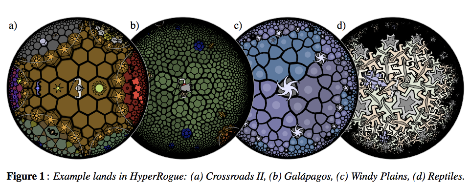
I recently needed to demonstrate this fact to an audience that I could not assume would be familiar with Riemannian geometry, and it took some time to find a way to do it! You can use the HyperRogue game, which takes place on a tiling of the Poincaré disc. The avatar moves across the Poincaré disc (slaying monsters and collecting treasure) by stepping from tile to tile. It is a pretty impressive piece of software, and you can play it on various devices for small change. Below are four scenes from the game. This image was taken from the interesting paper on HyperRogue by Kopczyński et al., cited at bottom.

As a proxy for proving that the growth rate was exponential, just count the number of tiles that were accessible (starting from the centre tile) in N steps and no less. This gives the sequence 1, 14, 28, 49, 84, 147, 252, 434, 749, … . Plotting this values gives evidence enough.

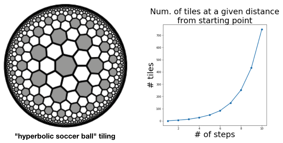
The authors of the paper do a more thorough job, obtaining a recurrence relation for the sequence and using this to derive the base of the exponential growth (which comes out at about $\sqrt{3}$.

[1] Kopczyński, Eryk; Celińska, Dorota; Čtrnáct, Marek. “HyperRogue: playing with hyperbolic geometry”. Proceedings of Bridges 2017: Mathematics, Music, Art, Architecture, Culture (2017).

Eurovision song contest dataset

I’m teaching hierarchical clustering in my course on DataCamp, and I needed an interesting dataset. Importantly, I wanted the dataset to have labelled instances, so that the dendrogram would be easily interpretable, but also not too many instances, so they all fit on the dendrogram. Fortunately for me, the Eurovision song contest has been publishing the voting results (which is great!) and these are perfect. Both the voting results from the judges, and those from the public give great results. The only thing you need to adjust for is that countries are not allowed to vote for themselves in Eurovision, and this gives you some missing values in the data. I filled these with the maximum score of 12, since it is reasonable to assume that countries would vote selfishly if they were allowed to. Below is the dendrogram of a hierarchical (agglomerative) clustering using complete linkage.

A better version

It occurs to me now that I should have normalised the rows after filling in the missing values. This does indeed improve the hierarchical clustering further.

Wine dataset demonstrates importance of feature scaling

The UCI hosts a dataset of wine measurements that is fantastic for demonstrating the importance of feature scaling in unsupervised learning . There are a bunch of real-valued measurements (of e.g. chemical composition) for three varieties of wine: Barolo, Grignolino and Barbera. I am using this dataset to introduce feature scaling my course on DataCamp.

The wine measurements have very different scales, and performing a k-means clustering (with 3 clusters) on the unscaled measurements yields clusters that don’t correspond to the varieties:

varieties  Barbera  Barolo  Grignolino
labels                                
0               29      13          20
1                0      46           1
2               19       0          50

However, if the measurements are first standardised, the clusters correspond almost perfectly to the three wine varieties:

varieties  Barbera  Barolo  Grignolino
labels                                
0                0      59           3
1               48       0           3
2                0       0          65

Of course, k-means clustering is not meant to be a classifier! But when the clusters do correspond so well to the classes, then it is apparent that the scaling is pretty good.

Which wine varieties?

I had to search to find the names of the wine varieties. According to page 9 of “Chemometrics with R” (Ron Wehrens), the three varieties are: Barolo (58 samples), Grignolino (71 samples) and Barbera (48 samples). I was unable to follow Wehren’s citation (it’s his [6]) on Google books.

Original source

According to the UCI page, this dataset originated from the paper V-PARVUS. An Extendible Pachage of programs for esplorative data analysis, classification and regression analysis by Forina, M., Lanteri, S. Armanino, C., Casolino, C., Casale, M., Oliveri, P.

Olive oil dataset

There is a dataset of olive oil measurements associated to the same paper. I haven’t tried using it, but am sure I’ll use it in an example one day.

An LCD digit dataset for illustrating the “parts-based” representation of NMF

Non-negative matrix factorisation (NMF) learns to reconstruct samples as a superposition of their constituent parts. In the paper of Lee and Seung (1999) that popularised NMF, this is called a “parts-based” representation. This is illustrated in that paper by applying NMF to encodings of images of faces, where NMF seems to decompose the faces into a collage of eigen-eyebrows and eigen-noses. Visual demonstrations are fantastic for conveying ideas, but in this particular instance, the clarity is compromised by the inherent noisiness of real-world facial images. The images are drawn, moreover, from the CBCL dataset, which has a non-commercial license. In order to get around this problem, and to have an even clearer visual demonstration of the “parts-based” decomposition provided by NMF for my course at DataCamp, I created a synthetic image dataset, where each image is of a single digit of a LCD display, as on a clock radio. The parts learned by NMF are then the individual “cells” of the LCD display.

You can construct this dataset yourself, using the code below. The collection of images is encoded as a 2d array of non-negative values. Each row corresponds to an image, and each column corresponds to a pixel. The non-negative entries represent the whiteness of the pixel, encoded here as a value between 0 and 1.

Alternatives

  • The standard bars provide a similar (but more apparently synthetic) image dataset for learning the parts of images. See, for example, the references given in Spratling (1996).
  • Another great visual dataset could be built from black-and-white images of the 52 playing cards in a deck. NMF would then learn the ranks (i.e. ace, 2, 3, …, ) and the suits (i.e. spades, hearts, …) as parts, and reconstruct playing cards from these. I haven’t done this.
  • Yet another great example dataset could be constructed using images of a piano keyboard, or perhaps just an octave range, colouring the keys according to how often they are pressed during a song. NMF should then be able to learn the chords as parts. The midi files to construct this dataset could be obtained from the Mutopia project, for example. I haven’t done this either.

Descartes’ headache: rotation of space is transpose to rotation of co-ordinate system

[I often speak of such-and-such depending upon the choice of co-ordinate system, and proceed to show this by rotating the space. The following explains why this is equivalent (via the transpose)].

You awaken in a two-dimensional landscape. In front of you are co-ordinate axes, fixed to the ground on a pivot. The landscape is featureless except for a tree and a well. You get bored, and fall asleep again. When you awaken, you notice that the relative arrangement of the co-ordinate axes to the tree and the well is different. What happened?

You realise that you’ll never truly know what happened while you were asleep. Either (a) someone rotated the co-ordinate axes 90 degrees clockwise, or (b) someone rotated the world 90 degrees anti-clockwise about the pivot point of the axes.

Rotation of the space is equivalent (via the transpose) to rotation of the co-ordinate system. In fact, this is true more generally for orthogonal transformations and has a familiar mathematical expression. Let $V$ be an n-dimensional vector space with inner product $\langle \cdot , \cdot \rangle$ and let $e_i, i=1, .., n$ be an orthonormal basis. If $X$ is an orthogonal transformation of $V$, then for any point $v \in V$, we have
$$ \displaystyle $\langle Xv, e_i \rangle = \langle v, X^T e_i \rangle $$

for all $i=1, .. , n$. That is, the co-ordinates of the transformed point with respect to the original basis are the co-ordinates of the original point with respect to the transpose-transformed basis.

Block Multiplication of Matrices

(We needed this to derive the conditional distribution of a multivariate Gaussian).

Consider a matrix product $AB$. Partition the two outer dimensions (i.e. the rows of $A$ and the columns of $B$) and the one inner dimension (i.e. the columns of $A$ and the rows of $B$) arbitrarily. This defines a “block decomposition” of the product $AB$ and of the factors $A, B$ such that the blocks of $AB$ are related to the blocks of $A$ and $B$ via the familiar formula for components of the product, i.e.

$(AB)_{m,n} = \sum_s A_{m,s} B_{s,n}$.

Pictorially, we have the following:

blockmultnmatrices

Arithmetically, this is easy to prove by considering the formula above for the components of the product. The partitioning of the outer dimensions comes for free, while the partitioning of the inner dimension just corresponds to partitioning the summation:

$(AB)_{m,n} = \sum_s A_{m,s} B_{s,n} = \sum_i \sum_{s_i \leq s \leq s_{i+1}} A_{m,s} B_{s,n}$.

Zooming out to a categorical level, we can see that there is nothing peculiar about this situation. If, in an additive category, we have three objects $X, Y, Z$ with biproduct decompositions, and a chain of morphisms:

$X \xrightarrow{\varphi_B} Y \xrightarrow{\varphi_A} Z$

then this “block decomposition of matrices” finds expression as a formula in $\text{End}(X, Z)$ using the injection and projection morphisms associated with each biproduct factor.