Deep Differentiable Logic Gate Networks & their (potential) relevance to ZKML

This paper (arXiv), authored by Petersen, Borgelt, Kuehne and Deussen, was accepted for NeurIPs 2022. It does one of my favourite things: it learns a discrete structure (in this case, a boolean circuit) via differentiable means. Logic gate networks came up in a recent ZKML discussion as a machine learning paradigm of interest: since boolean circuits are encodable as arithmetic circuits, proving inference runs of a logic gate network can be done without the loss of accuracy that is inherent in the quantization approach to making the more familiar neural nets amenable to ZK. In fact, the situation is more subtle than that: a logic gate network is in fact discretized before inference (just not by us), and there was necessarily a small loss in accuracy in that process. An important difference, however, is that logic gate networks have been designed with this discretization in mind, since this is exactly what needs to be done to make model inference fast on edge hardware. This post presents notes on a presentation on this topic and the questions that arose during the discussion.

What’s a deep differentiable logic gate network?

A differentiable logic gate network consists of multiple layers of “neurons” with random wiring:

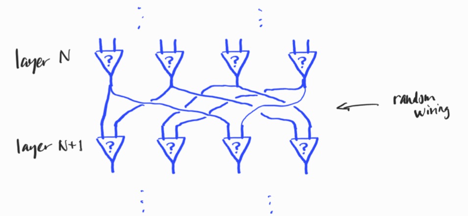
Each neuron has precisely two inputs and is a superposition of the possible binary logic gates:

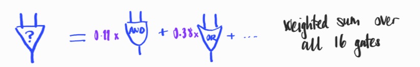
where the probabilities (in purple) are learned from the data (using the softmax parameterization).

During training, the logic gates operate on values in the interval $[0,1]$ via arithmetic expressions e.g. $$\mathrm{OR}(x,y) = x + y – xy,$$and the output of a neuron is the expected value, over all logic gates, of their respective outputs, i.e. it’s a sum of the outputs of each gate, weighted by the probability of that gate (the purple values). Post-training, the network is discretized to yield a boolean circuit by replacing each neuron with its most likely logic gate.

Novelty

The superposition of different architectural components (logic gates) via the softmax is, to the best of my knowledge, novel. Note that here, softmax is not an activation function. Moreover, it’s not similar to the use of softmax in attention, as the probabilities are independent of the current input.

Points of interest

Why all 16 possible gates?

There are 16 possible binary logic gates – just count the boolean functions of two variables. Even though a smaller variety of gates would suffice to express any boolean circuit, the authors allow all 16, and this at the expense of increasing the training time, since there are more outcomes in the softmax to parameterise. The authors talk about this in the paper themselves. However, very deep circuits are hard to learn in their regime, so this redundancy is purposeful here.

Deep(er) logic gate networks are hard to learn

The authors explain this in terms of vanishing gradients. I think the problem is more fundamental, having nothing to do with the gradient, per se. An expectation is taken at every neuron/node in the circuit, and the layering of these successive expectations means that the signal at the output layer is very diluted. It is interesting to reflect that what we really would like to do is perform a superposition over all possible circuits of some size. This is of course infeasible, since the number of such circuits would be astronomical. So the authors perform superpositions of logic gates at each node, instead. Since deep logic gate networks are hard to learn (the maximum depth used by the authors is 6 layers), the authors go wide: their largest network has 1M nodes on each layer!

The wiring is fixed

The wiring of the network is the pattern of connections from layer to layer. Familiar neural networks are often fully connected, so each neuron is connected to all neurons in the previous layer. For logic gate networks, this is not the case: each neuron receives precisely two inputs from the outputs of the previous layer. There are obviously a huge number of choices for how to wire two layers together. In the approach of the authors, for simplicity, the wiring is determined pseudo-randomly before training and fixed for all time.

The authors don’t count the connection information in the storage requirements for the model, since the connections are determined by the initial random seed. This isn’t wrong, but it’s worth remembering (as the authors themselves note) that any future approach that employs a more intelligent method of determining the wiring will need to store the connection information.

Learning the wiring would be better

Learning the wiring would likely mean (in my estimation) that the such wide layers wouldn’t be necessary: a huge number of random connections would no longer be required to find the favourable information flows from inputs to outputs. Learning the wiring would be a non-trivial optimisation problem, however, more complicated than e.g. general sparsity constraints since the number of inputs must be exactly two (not just a arbitrary small number).

Regression as well as classification?

The authors also undertake to demonstrate that logic gate networks, when appended with a learned affine transformation, are useful devices for regression. This is not without precedent, since e.g. sometimes random forests are used for regression. However, I think the core case of classification is compelling enough.

The “normalisation temperature” $\tau$

Outputs are grouped into equally sized groups corresponding to the classes of the classification, and the score for each class is the sum of its outputs. These sums need normalising, since the resultant “score vector” needs to be a distribution: it is compared to the target distribution (which is one-hot on the target class) using cross entropy. There is only one correct way to do this, namely normalize by the size of the groups. Instead, the authors normalize by a hyperparameter $\tau$, for which they perform a grid search. The beneficial side effect of varying the value of $\tau$ is to amplify or diminish the strength of the back propagation signal, and as such, it ends up playing the role of a learning rate (the hyperparameter that the authors identify as a learning rate is in fact fixed).

Surprisingly, no annealing!

It is common practice to use a “temperature” parameter in the softmax to progressively encourage the model to move towards making a one-hot decision – this is called annealing. Surprisingly, the authors choose not to do this, and perhaps they didn’t need to (see Discretization).

Discretization

The authors claim that, post-training, the model has learned an unambiguous choice of logic gate for each node; they are consequently able to discretize the network of superpositions into a boolean circuit. This of course damages the accuracy of the model. The authors report however that this lose of accuracy is less that 0.1% for MNIST.

(I was skeptical about the claim that the choice of logic gate would be unambiguous post training, but can confirm that this is indeed the case: after training the smaller MNIST model, >96% of all neurons on all layers were essentially one-hot (i.e. one outcome had probability >85%).

Relevance to ZKML

Logic gate networks belong to the broad family of approaches that are focussed on efficient inference for edge devices, which includes further model types that may be of interest for ZKML, such as binary neural nets, quantised weight networks and neural nets trained with sparsity constraints. The other feature that all such models have in common is that they sacrifice some accuracy for efficiency and are consequently never the latest and greatest in performance. However, logic gate networks in particular are still in the first stages of their development, and future directions for improvement are apparent and, in my opinion, feasible.

The most important future improvement will be lower redundancy. Logic gate networks (in their current state) are boolean circuits with a high degree of redundancy resulting from their learning process. Reducing this redundancy will be crucial for making such models useful beyong toy datasets. For example, about four million logic gates are required for a competitive logic gate network for MNIST. From the ZKML perspective, to prove an inference run of such a network, the output of each logic gate (a bit) needs to be encoded as a separate field element – they can’t be grouped together into a larger field element since bit-wise operations need to be verified. While this is not so onerous (depending on the proof system), this is still just a model for a toy dataset. What is needed is a method of learning with reduced redundancy, and this will hopefully be the result of future work.

Improving Pairwise Learning for Item Recommendation from Implicit Feedback 2014

Steffen Rendle and Christoph Freudenthaler (University of Konstanz), WSDM 2014.
The authors present a modification of the Bayesian Pairwise Ranking (BPR) for implicit feedback (i.e. one class) recommendation datasets in which the negative samples are drawn according both to the models current belief and the user/context in question (“adaptive oversampling“). They show that the prediction accuracy of BPR models trained with adaptive oversampling matches that of BPR models trained with uniform sampling but that convergence is 10x-20x faster.
Consider the problem of recommending items to users (or more generally: contexts, e.g. user on a particular page).  The observed data consists then of context-item pairs $(c, i)$, where item $i$ was the choice made in context $c$.  The authors work in the context of pairwise learning, which amounts to a binary classification task where context-item-item triples $(c, i, j)$ are labelled as true i.f.f. item $i$ was chosen in context $c$ but item $j$ is not:
Screen Shot 2016-03-21 at 11.54.46
where $\hat{y}$ is a scoring function (e.g. the dot product of the context- and the item- latent vectors, for matrix factorisation).  It is infeasible to consider all the negative examples $j$, so how should we choose which to consider?

Negative sampling from static distributions

We could draw negative examples from the uniform distribution over all items, or instead from the observed distribution over all items (i.e. by popularity).  Both are inexpensive to perform and easy to implement.  However:
  • Uniform sampling tends to yield uninformative samples, i.e. those for which the probability of being incorrectly labelled is very likely already low: popular items are precisely those that appear often as positive examples (and hence tend to be highly ranked by the model), while a uniformly-drawn item is likely to be from the tail of the popularity distribution (so likely lowly ranked by the model).
  • Sampling according to popularity is demonstrated by the authors to converge to inferior solutions.
The authors point out that these sampling schemes depend neither upon the current context (user) nor the current belief of the model.  This contrasts with their own method, adaptive over-sampling.

Adaptive over-sampling

The authors propose a scheme in which the negative samples chosen are those that the model would be likely to recommend to the user in question, according to its current state.  In this sense it is reminiscent of the Gibbs sampling used by restricted Boltzmann machines.
Choosing negative samples dependent on the current model and user is computationally expensive if performed in the naive manner. The authors speed this up by working with the latent factors individually, and only periodically re-computing the ranking of the items according to each latent factor.  Specifically, in the case of matrix factorisation, when looking for negative samples for a context $c$, a negative sample is chosen by:
  1. sampling a latent factor $l$ according to the absolute values of the latent vector associated to $c$ (normalised, so it looks like a probability distribution);
  2. sampling an item $j$ that ranks highly for $l$.  More precisely, sample a rank $r$ from a geometric distribution over possible ranks, then find the item that has rank $r$ when the $l$th coordinates of the item latent vectors are compared.

(We have ignored the sign of the latent factor.  If the sign is negative, one choses the rth-to-last ranked item).  The ranking of the items according to each latent factor is precomputed periodically with a period such that the extra overhead is independent of the number of items (i.e. is a constant).

Problems with the approach

The samples yielded by the adaptive oversampling approach depend heavily upon the choice of basis for the latent space.  It is easy to construct examples of where things go wrong:

Non-negativity constraints would solve this.  Regularisation would also deal with this particular example – however regularisation would complicate the expression of the scoring function $\hat y$ as a mixture (since you need to divide though by $Z_c$.

Despite these problems, the authors demonstrate impressive performance, as we’ll see below.


Performance

The authors demonstrate that their method does converge to solutions slightly better than those given by uniform sampling, but twenty times faster.  It is also interesting to note that uniform sampling is vastly superior to popularity based sampling, as shown in the diagrams below.
Screen Shot 2016-03-21 at 11.54.01
Note that a single epoch of the adaptive oversampling takes approximately 33% longer than a single epoch of uniform sampling BPR.

Implementation

According to the paper, the method is implemented in libFM, a C++ software package that Rendle has published.  However, while I haven’t looked exhaustively, I can’t see anything in that package about the adaptive oversampling (nor in Rendle’s other package, MyMediaLite).


What about adaptive oversampling in word2vec?

Word2vec with negative sampling learns a word embedding via binary classification task, specifically, “does the word appear in the same window as the context, or not?”.  As in the case of implicit feedback recommendation, the observed data for word2vec is one-class (just a sequence of words).  Interestingly, word2vec samples from a modification of the observed word frequency distribution (i.e. of the “distribution according to popularity”) in which the frequencies are raised to the $0.75$th power and renormalised.  The exponent was chosen empirically.  This raises two questions:

  1. Would word2vec perform better with adaptive oversampling?
  2. How does BPR perform when sampling from a similarly-modified item popularity distribution (i.e. raising to some exponent)?


Corrections

Corrections and comments are most welcome. Please get in touch either via the comments below or via email.


WARP loss for implicit-feedback recommendation

We consider the “Weighted Approximate-Rank Pairwise-” (WARP-) loss, as introduced in the WSABIE paper of Weston et. al (2011, see references), in the context of making recommendations using implicit feedback data, where it has been shown several times to perform excellently.  For the sake of discussion, consider the problem of recommending items $i$ to users $u$, where a scoring function $f_u(i)$ gives the score of item $i$ for user $u$, and the item with the highest score is recommended.

WARP considers each observed user-item interaction $(u, i)$ in turn, choses another “negative” item $i’$ that the model believed was more appropriate to the user, and performs gradient updates to the model parameters associated to $u$, $i$ and $i’$ such that the models beliefs are corrected.  WARP weights the gradient updates using (a function of) the estimated rank of item $i$ for user $u$.  Thus the updates are amplified if the model did not believe that the interaction $(u, i)$ could ever occur, and are dampened if, on the other hand, if the interaction is not surprising to the model. Conveniently, the rank of $i$ for $u$ can be estimated by counting the number of sample items $i’$ that had to be considered before one was found that the model (erroneously) believed more appropriate for user $u$.

Minimising the rank?

Ideally we would like to make updates to the model parameters that minimised the rank of item $i$ for user $u$.  Previous work of Usunier (one of the authors) showed that the precision at k was best optimised when the logarithm of the rank was minimised.  (to read!)

The problem with the rank is that, while it does depend on the model parameters, this dependence is not continuous (the rank being integer valued!).  So it is not possible to speak of gradients.  So what is to be done instead?  The approach of the authors is to derive a differentiable approximation to the logarithm of the rank, and to minimise this instead.

Derivation: approximating the (log of the) rank

WARP has been shown several times to perform very well for implicit feedback recommendation.  However, the derivation of the approximation of the log of the rank used in WARP, as outlined in the WSABIE paper, is nonsense.  I can only think that the authors arrived at WARP in another way.  Let’s look at it more closely.  In the following:

  • $f_u (i)$ is the score assigned by the model to item $i$ for user $u$.
  • $L$ is some function that defines the error as a function of the rank.  In the WSABIE paper, $L(k) = \sum_{j=1}^k \frac{1}{j}$ is approximately the natural logarithm (for the derivation below, however, it doesn’t matter what $L$ is)

warp derivation
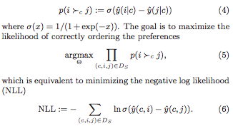
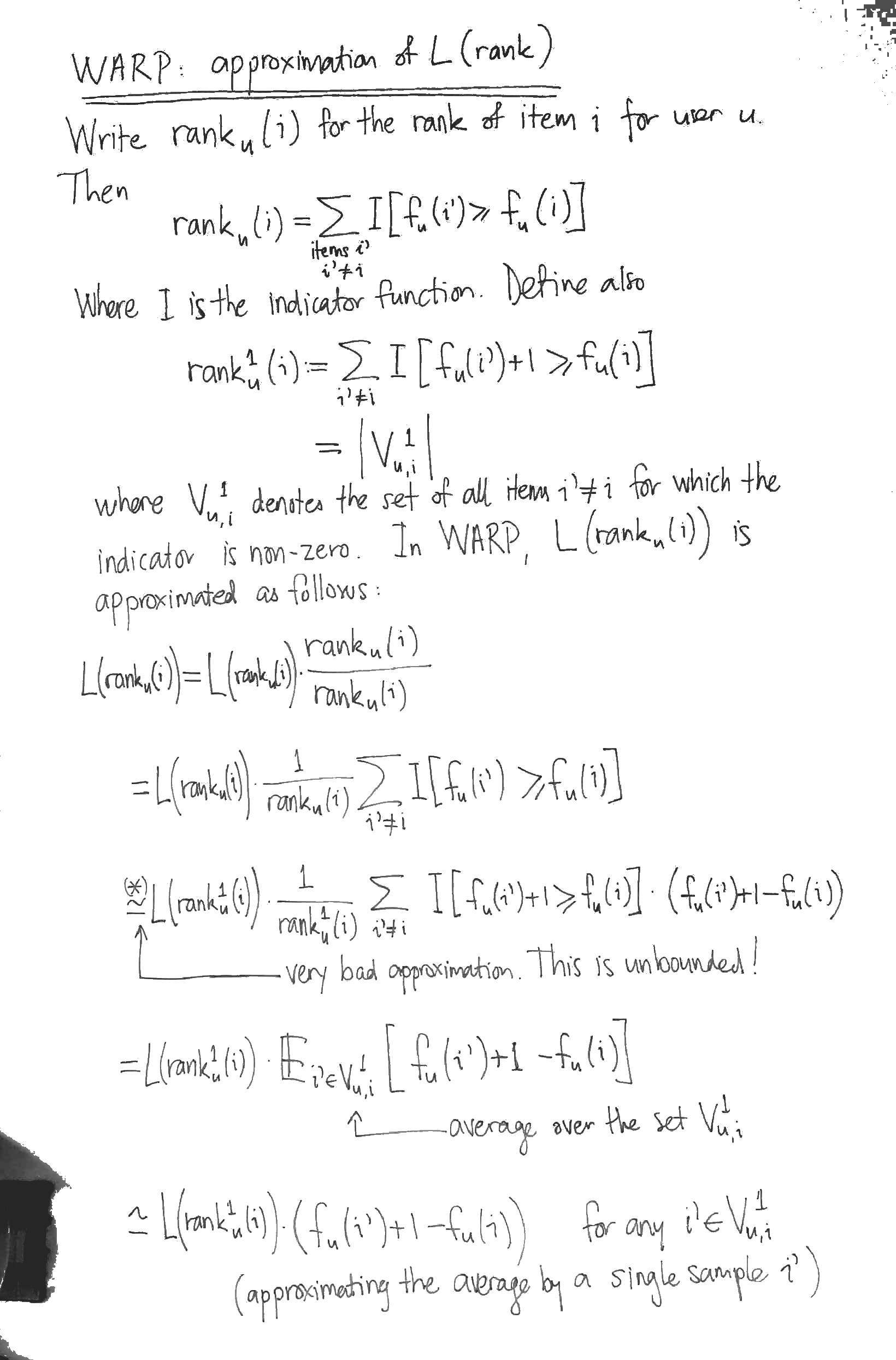
The most obvious problem with the derivation is the approximation marked with an asterix (*).  At this step, the authors approximate the indication function $I[x > y]$ by $I[x > y] \cdot (x – y + 1)$.  While the latter is familiar as the hinge loss from SVMs, it is (begin unbounded!) a dreadful approximation for the indicator $I[x > y]$.  It seems to me that the sigmoid of the difference of the scores would be a much better differentiable approximation to the indicator function.

To appreciate why the derivation is nonsense, however, you have to notice that the it has nothing to do with $L$.  That is, the derivation above would yield an approximation for $L$, whatever $L$ happened to be, even a constant function.

Optimisation

WARP considers each observed interaction $(u, i)$ in turn, repeatedly sampling items $i’$ from the uniform distribution over all items until it finds one in $V_{u, i}^1$, i.e. until it finds an item $i’$ whose score for the user $u$ is at worst 1 less than the score of the observed interaction.  For this triple $(u, i, i’)$, it performs gradient updates to minimise:

$\displaystyle L( \text{rank}_u^1 (i) ) \cdot (f_u (i’) + 1 – f_u (i))$

The naive approach to computing $\text{rank}_u^1 (i)$ is to calculate all the scores for the given user in order to determine the rank of the item $i$.  WARP performs a nice trick to do much better: it estimates $\text{rank}_u^1 (i)$ by counting how many candidate negative items $i’$ it had to consider before finding one in $V_{u, i}^1$.  This yields

$\displaystyle \text{rank}_u^1 (i) \approx \frac{\text{total number of items} – 1}{\text{number of i’ we had to draw}}$

However it is still the case that $L(\text{rank}_u^1 (i))$ is not differentiable.  So when we compute the gradients, this quantity has to be treated as a constant. Thus it simply becomes a weighting applied to the gradient of the difference of the scores (hence the name WARP, I guess).

WARP optimises for item to user recommendations

With its negative sampling technique, WARP optimises for recommending items to a user.  For instance, the problem of recommending users to items (so, transposing the interaction matrix) is not trained for.  I wonder if some extra uplift could be obtained by training for both problems simultaneously.

Normalising for the total number of items

With the optimisation stated as above, the learning rate will need to be re-tuned for datasets that have different numbers of items, since the gradient weighting $L( \text{rank}_u^1 (i) )$ is ranges from $L(0)$ to $L(\text{total number items})$.  It would make more sense to weigh the gradient updates by:

$\displaystyle \frac{L( \text{rank}_u^1 (i) )}{L(\text{total number items})}$

which ranges between 0 and 1.

Implementations

There are two implementations of WARP for recommendation that I know of, both in Python:

  • LightFM, written by Maciej Kula.  Works well.  Also implements BPR with uniform sampling and WARP k-OS (which I’ve not investigated yet).
  • MREC, written by Levy and Jack at Mendeley, has a matrix factorisation recommender trained using WARP.  I’ve not tried this one out yet.

References

Jason Weston, Samy Bengio and Nicolas Usunier, Wsabie: Scaling Up To Large Vocabulary Image Annotation, 2011, (PDF).

GloVe: Global Vectors for Word Representations

Pennington, Socher, Manning, 2014.
PDF

GloVe trains word embeddings by performing a weighted factorisation of the log of the word co-occurrence matrix. The model scales to very large corpora (Common Crawl 840B tokens) and performs well on word analogy tasks.

Model
The cost function is given by:

$\displaystyle \sum_{i, j = 1}^V f(X_{i,j}) (u_i^T v_j + b_i + c_j – \text{log} X_{i,j})^2$

where:

  • $V$ is the size of the vocabulary,
  • $X$ denotes the word co-occurrence matrix (so $X_{i,j}$ is the number of times that word $j$ occurs in the context of word $i$)
  • the weighting $f$ is given by $f(x) = (x / x_{\text{max}})^\alpha$ if $x < x_{\text{max}}$ and $1$ otherwise,
  • $x_{\text{max}} = 100$ and $\alpha = 0.75$ (determined empirically),
  • $u_i, v_j$ are the two layers of word vectors,
  • $b_i, c_j$ are bias terms.

Note that the product is only over pairs $i, j$ for which $X_{i,j}$ is non-zero. This means that GloVe (in contrast to word2vec with negative sampling) trains only “positive samples” and also that we don’t have to worry about the logarithm of zero.

This is essentially just weighted matrix factorisation with bias terms:

glove-matrix-factorisation

Note that in the implementation (see below), the $X_{i,j}$ are not raw co-occurrence counts, but rather the accumulated inverse distance between the two words, i.e.

$\displaystyle X_{w, w’} := \sum_{\text{windows containing\ } w, w’} (\text{distance between\ } w, w’)^{-1}.$

I am fairly sure that the implementation of Adagrad is incorrect. See my post to the forum.

The factor weighting f

The authors go to some trouble to motivate the definition of this cost function (section 3).  The authors note that many different functions could be used in place of their particular choice of $f$, and further that their $\alpha$ coincides with that used by word2vec for negative sampling. I can’t see the relevance of the latter, however (in word2vec, the $0.75$th power it is used to define the noise distribution; moreover powering a value in the range $[0, 1]$ has a very different effect to powering a value in the range $[0, 100]$).

glove-weighting-function

Graphing the function (see above) hints that it might have been specified more simply, since the non-linear region is in fact almost linear.

A radial window size of 10 is used. Adagrad is used for optimisation.

Word vectors
The resulting word embeddings ($u_i$ and $v_j$) are unified via a direct sum of their vector spaces.

The cosine similarity is used to find the missing word in word similarity tasks. It is not stated if the word vectors were normalised before forming the arithmetic combination of word vectors.

Source code
The authors take the exemplary step of making the source code available.

Evaluation and comparison with word2vec
The authors do a good job of demonstrating their approach, but do a scandalously bad job of comparing their approach to word2vec. This seems to reflect a profound misunderstanding on the part of the authors as to how word2vec works. While it has to be admitted that the word2vec papers were not well written, it is apparent that the authors made very little effort at all.

The greatest injustice is the comparison of the performance of GloVe with an increasing number of iterations to word2vec with an increasing number of negative samples:

The most important remaining variable to control
for is training time. For GloVe, the relevant
parameter is the number of training iterations.
For word2vec, the obvious choice would be the
number of training epochs. Unfortunately, the
code is currently designed for only a single epoch:
it specifies a learning schedule specific to a single
pass through the data, making a modification for
multiple passes a non-trivial task. Another choice
is to vary the number of negative samples. Adding
negative samples effectively increases the number
of training words seen by the model, so in some
ways it is analogous to extra epochs.

Firstly, it is simply impossible that it didn’t occur to the authors to simulate extra iterations through the training corpus for word2vec by simply concatenating the training corpus with itself multiple times. Moreover, the authors themselves are capable programmers (as demonstrated by their own implementation). The modification to word2vec that they avoided is the work of ten minutes.

Secondly, the notion that increasing the exposure of word2vec to noise is comparable to increasing the exposure of GloVe to training data is ridiculous. The authors clearly didn’t take the time to understand the model they were at pains to criticise.

While some objections were raised about the evaluation performed in this article and subsequent revisions have been made, the GloVe iterations vs word2vec negative sample counts evaluation persists in the current version of the paper.

Another problem with the evaluation is that the GloVe word vectors formed as the direct sum of the word vectors resulting from each matrix factor. The authors do not do word2vec the favour of also direct summing the word vectors from the first and second layers.

Links

Document Embedding with Paragraph Vectors

Presented at NIPS 2014 (PDF) by Dai, Olah, Le and Corrado.

Model

The authors consider a modified version of the PV-DBOW paragraph vector model. In previous work, PV-DBOW had distinguished words appearing in the context window from non-appearing words given only the paragraph vector as input. In this modified version, the word vectors and the paragraph vectors take turns playing the role of the input, and word vectors and paragraph vectors are trained together. That is, a gradient update is performed for the paragraph vector in the manner of regular PV-DBOW, then a gradient update is made to the word vectors in the manner of Skipgram, and so on. This is unfortunately less than clear from the paper. The authors were good enough to confirm this via correspondence, however (thanks to Adriaan Schakel for communicating this). For the purposes of the paper, this is the paragraph vector model.

The representations obtained from paragraph vector (using cosine similarity) are compared to those obtained using:

  • an average of word embeddings
  • LDA, using Hellinger distance (which is proportional to the L2 distance between the component-wise square roots)
  • paragraph vector with static, pre-trained word vectors

In the case of the average of word embeddings, the word vectors were not normalised prior to taking the average (confirmed by correspondence).

Corpora

Two corpora are considered, the arXiv and Wikipedia:

  • 4.5M articles from Wikipedia, with a vocabulary of size 915k
  • 886k articles from the arXiv, full texts extracted from the PDFs, with a vocabulary of 970k words.

Only unigrams are used. The authors observed that bigrams did not improve the quality of the paragraph vectors. (p3)

Quantitative Evaluation

Performance was measured against collections of triples, where each triple consisted of a test article, an article relevant to the test article, and an article less relevant to the test article. While not explicitly stated, it is reasonable to assume that the accuracy is then taken to be the rate at which similarity according to the model coincides with relevance, i.e. the rate at which the model says that the relevant article is more similar than the less relevant article to the test article. Different sets of triples were considered, the graph below shows performance of the different methods relative to a set of 172 Wikipedia triples that the authors built by hand (these remain unreleased at the time of writing).

Screen Shot 2015-05-24 at 15.23.52

It is curious that, with the exception of the averaged word embeddings, the accuracy does not seem to saturate as the dimension increases for any of the methods. However, as each data point is the accuracy of a single training (confirmed by correspondence), this is likely nothing more than the variability inherent to each method. It might suggest, for example, that the paragraph vectors method has a tendency to get stuck in local minima. This instability in paragraph vector is not apparent, however, when tested on the triples that are automatically generated from Wikipedia (Figure 5). In this latter case, there are many more triples.

Performance on the arXiv is even more curious: accuracy decreases markedly as the dimension increases!

Screen Shot 2015-05-24 at 15.24.39

Implementations

I am not sure there are any publicly available implementations of this modified paragraph vectors method. According to Dai, the implementation of the authors uses Google proprietary code and is unlikely to be released. However it should be simple to modify the word2vec code to train the paragraph vectors, though some extra code will need to be written to infer paragraph vectors after training has finished.

I believe that the gensim implementation provides only the unmodified version of PV-DBOW, not the one considered in this paper.

Comments

It is interesting that the paragraph vector is chosen so as to best predict the constituent words, i.e. it is inferred. This is a much better approach from the point of view of word sense disambiguation than obtaining the paragraph vector as a linear image of an average of the word vectors (NMF vs PCA, in their dimension reductions on bag of words, is another example of this difference).

Thanks to Andrew Dai and Adriaan Schakel for answering questions!

Questions

  1. Is there is an implementation available in GenSim? (see e.g. this tutorial).
  2. (Tangent) What is the motivation (probabilistic meaning) for the Hellinger distance?