Language modeling – Building Babylon

12 May 201618 May 2023

Skipgram isn't Matrix Factorisation

The paper Neural Word Embeddings as Implicit Matrix Factorization of Levy and Goldberg was published in the proceedings of NIPS 2014 (pdf). It claims to demonstrate that Mikolov’s Skipgram model with negative sampling is implicitly factorising the matrix of pointwise mutual information (PMI) of the word/context pairs, shifted by a global constant. Although the paper is interesting and worth reading, it greatly overstates what is actually established, which can be summarised as follows:

Suppose that the dimension of the Skipgram word embedding is at least as large as the vocabulary. Then if the matrices of parameters $(W, C)$ minimise the Skipgram objective, and the rows of $W$ or the columns of $C$ are linearly independent, then the matrix product $WC$ is the PMI matrix shifted by a global constant.

This is a really nice result, but it certainly doesn’t show that Skipgram is performing (even implicitly) matrix factorisation. Rather it shows that the two learning tasks have the same global optimum – and even this is only shown when the dimension is larger than the vocabulary, which is precisely the case where Skipgram is uninteresting.

The linear independence assumption

The authors (perhaps unknowingly) implicitly assume that the word vectors on one of the two layers of the Skipgram model are linearly independent. This is a stronger assumption than what the authors explicitly assume, which is that the dimension of the hidden layer is at least as large as the vocabulary. It is also not a very natural assumption, since Skipgram is interesting to us precisely because it captures word analogies in word vector arithmetic, which are linear dependencies between the word vectors! This is not a deal breaker, however, since these linear dependencies are only ever approximate.

In order to see where the assumption arises, first recall some notation of the paper:

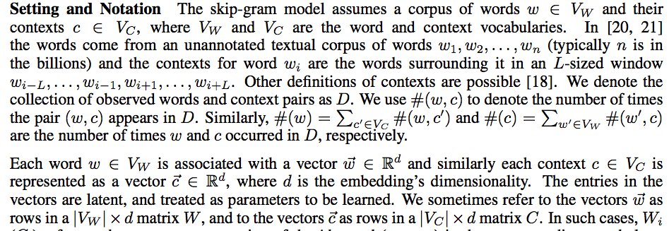
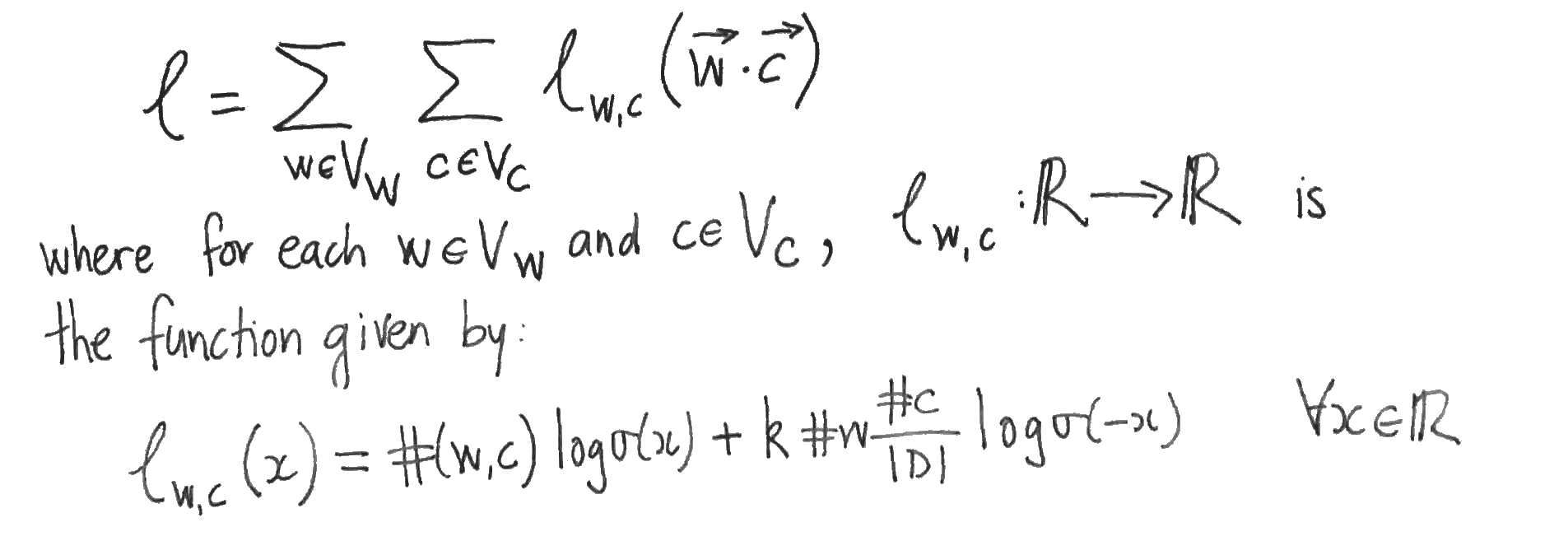
The authors consider the case where the negative samples for Skipgram are drawn from the uniform distribution $P_D$ over the contexts $V_C$, and write

for the log likelihood. The log likelihood is then rewritten as another double summation, in which each summand (as a function of the model parameters) depends only upon the dot product of one word vector with one context vector:

The authors then suppose that the values of the parameters $W, C$ are such that Skipgram is at equilibrium, i.e. that the partial derivatives of $l$ with respect to each word- and content-vector component vanish. They then assume that this implies that the partial derivatives of $l$ with respect to the dot products vanish also. To see that this doesn’t necessarily follow, apply the chain rule to the partial derivatives:

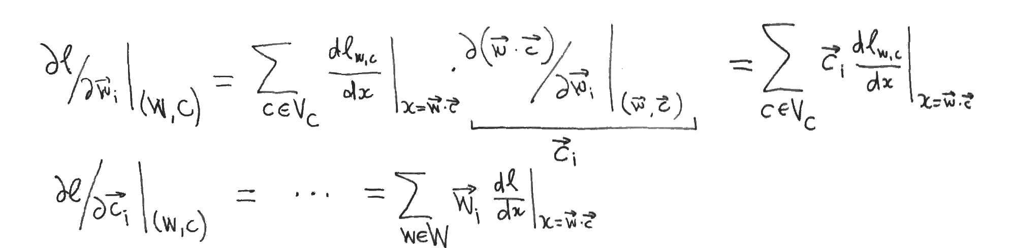
This yields systems of linear equations relating the partial derivatives with respect to the word- and content- vector components (which are zero by supposition) to the partial derivatives with respect to the dot products, which we want to show are zero. But this only follows if one of the two systems of linear equations has a unique solution, which is precisely when its matrix of coefficients (which are just word- or context- vector components) has linearly independent rows or columns. So either the family of word vectors or the family of context vectors must be linearly independent in order for the authors to proceed to their conclusion.

Word vectors that are of dimension the size of the vocabulary and linearly independent sound to me more akin to a one-hot or bag of words representations than to Skipgram word vectors.

Skipgram isn’t Matrix Factorisation (yet)

If Skipgram is matrix factorisation, then it isn’t shown in this paper. What has been shown is that the optima of the two methods coincide when the dimension is larger that the size of the vocabulary. Unfortunately, this tells us nothing about the lower dimensional case where Skipgram is actually interesting. In the lower dimensional case, the argument of the authors can’t be applied, since it is then impossible for the word- or context- vectors to be linearly independent. It is only in the lower dimensional case that the Skipgram and Matrix Factorisation are forced to compress the word co-occurrence information and thereby learn anything at all. This compression is necessarily lossy (since there are insufficient parameters) and there is nothing in the paper to suggest that the two methods will retain the same information (which is what it means to say that the two methods are the same).

Appendix: Comparing the objectives

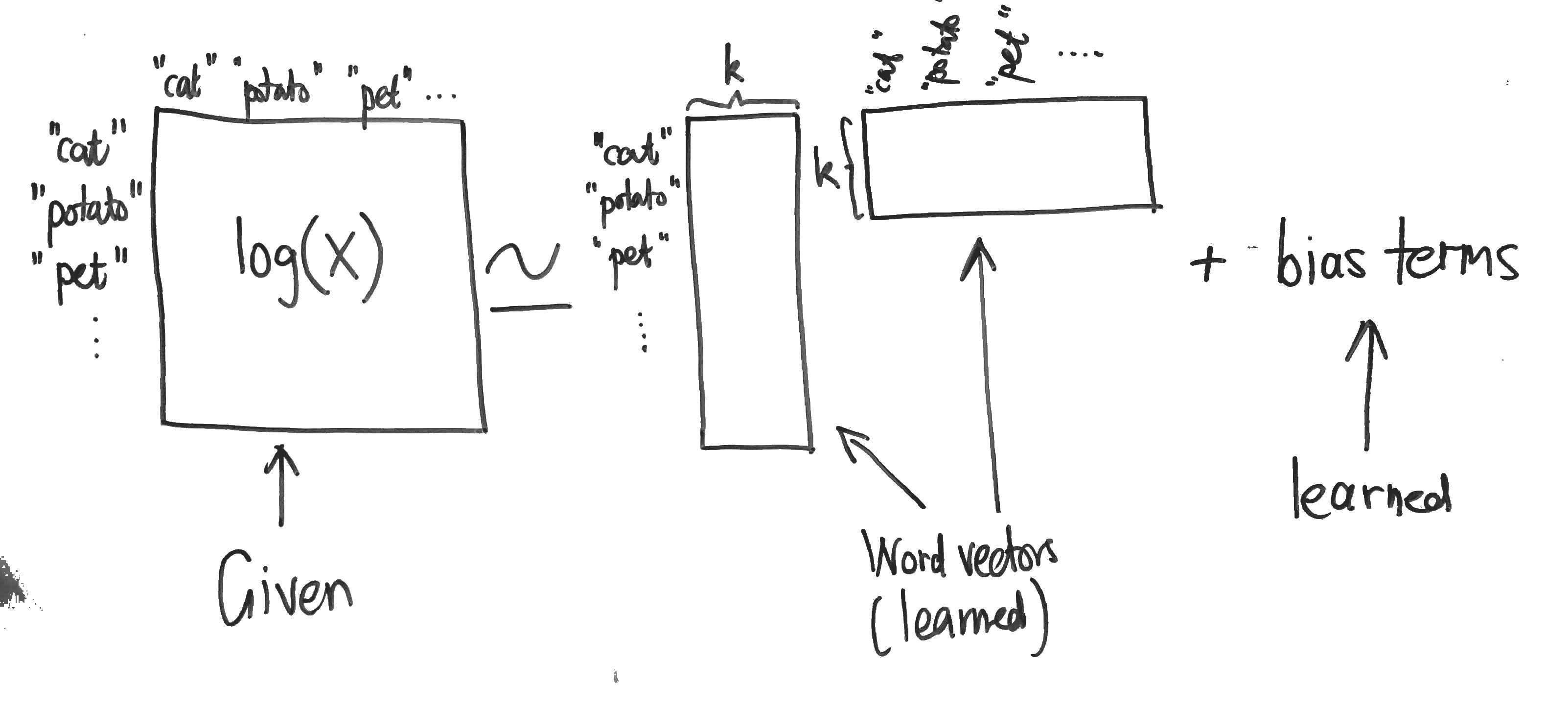
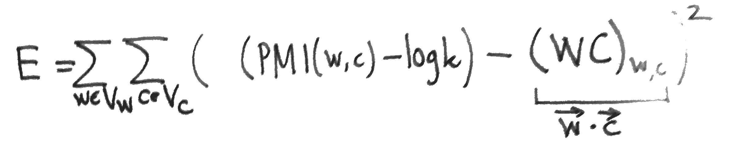
To compare Skipgram with negative sampling to MF, we might compare the two objective functions. Skipgram maximises the log likelihood $l$ (above). MF, on the other hand, typically minimises the squared error between the matrix and its reconstruction:

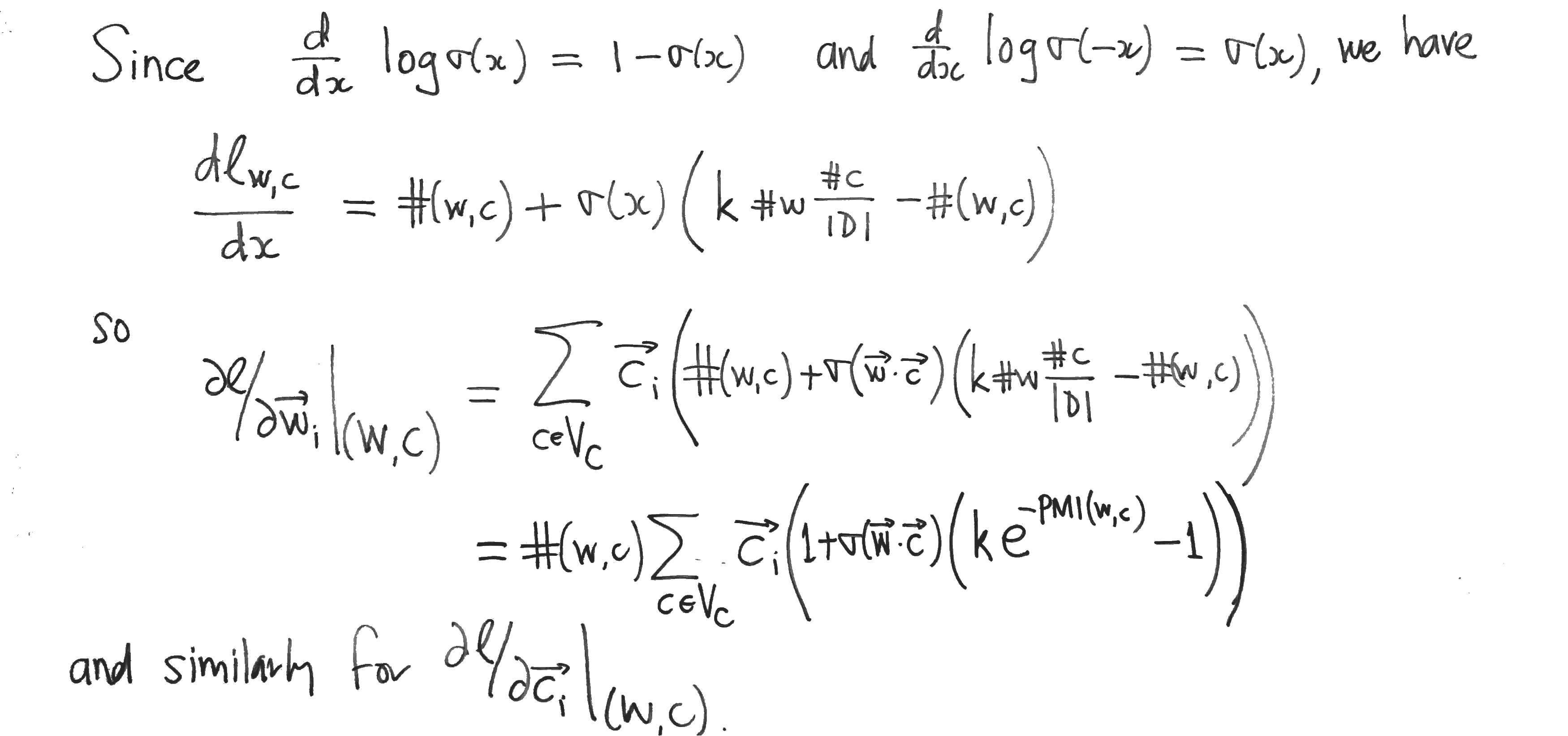
The partial derivatives of $E$, needed for a gradient update, are easy to compute:

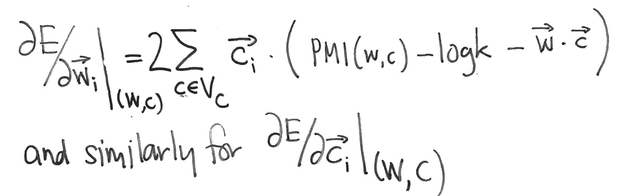
Compare these with the partial derivatives of the Skipgram log-likehood $l$, which can be computed as follows:

4 November 20158 May 2023

Does vector direction encode word frequency?

In a paper with Adriaan Schakel, we presented controlled experiments for word embeddings using pseudo-words. Performing these experiments in the case of word2vec CBOW showed that, in particular, the vector direction of any particular word changed only moderately when the frequency of the word was varied. Shortly before we released the paper, Schnabel et al presented an interesting paper at EMNLP, where (amongst other things), they showed that it was possible to distinguish rare from frequent words using logistic regression on the normalised word vectors, i.e. they showed that vector direction does approximately encode coarse (i.e. binary, rare vs. frequent) frequency information. Here, I wanted to quickly report that the result of Schnabel et al. holds for the vectors obtained from our experiments, as they should. Below, I’ll walk through exactly what I checked.

I took the word vectors that we trained during our experiments. You can check our paper for a detailed account. In brief, we trained a word2vec CBOW model on popular Wikipedia pages with a hidden layer of size 100, negative sampling with 5 negative samples, a window size of 10, a minimum frequency of 128, and 10 passes through the corpus. Sub-sampling was not used so that the influence of word frequency could be more clearly discerned. There were 81k unigrams in the vocabulary. Then:

the word vectors were normalised so that their (Euclidean-) length was 1.
the frequency threshold of 5000 was chosen (somewhat arbitrarily) to define the boundary between rare and frequent words. This gave 8428 “frequent” words. A random sample of the same size of the remaining “rare” words was then chosen, so that the two classes, “rare” and “frequent”, were balanced. This yielded approximately 17k data points, where a data point is a normalised word vector labelled with either “frequent” (1) or “rare” (0).
the data points were split into training- and test- sets, with 70% of the data points in the training set.
a logistic regression model was fit on the training set. An intercept was fit, but this boosted the performance only slightly. No regularisation was used since the number of training examples wass high compared to the number of parameters.
The performance on the test set was assessed by calculating the ROC curve on the training and test sets and the accuracy on the test set.

Model performance
Consider the ROC curve below. We see from that fact that the test curve approximately tracks the training curve that the model generalises reasonably to unseen data. We see also from the closeness of the curves to the axes at the beginning and the end that the model is very accurate in detecting frequent words when it gives a high probability (bottom left of the curve) and at detecting infrequent words when it gives a low probability (top right).

(ROC curve made using a helpful code snippet from sklearn)

The accuracy of the model on the test set was 82%, which agrees very nicely with what was reported in Schnabel et al., summarised in the following image:

The training corpus and parameters of Schnabel, though not reported in full detail (they had a lot of other things to report), seem similar. We know that their CBOW model was 50 dimensional, had a vocabulary of 103k words, and was trained on the 2008 Wikipedia.

29 July 201518 May 2023

GloVe: Global Vectors for Word Representations

Pennington, Socher, Manning, 2014.
PDF

GloVe trains word embeddings by performing a weighted factorisation of the log of the word co-occurrence matrix. The model scales to very large corpora (Common Crawl 840B tokens) and performs well on word analogy tasks.

Model
The cost function is given by:

$\displaystyle \sum_{i, j = 1}^V f(X_{i,j}) (u_i^T v_j + b_i + c_j – \text{log} X_{i,j})^2$

where:

$V$ is the size of the vocabulary,
$X$ denotes the word co-occurrence matrix (so $X_{i,j}$ is the number of times that word $j$ occurs in the context of word $i$)
the weighting $f$ is given by $f(x) = (x / x_{\text{max}})^\alpha$ if $x < x_{\text{max}}$ and $1$ otherwise,
$x_{\text{max}} = 100$ and $\alpha = 0.75$ (determined empirically),
$u_i, v_j$ are the two layers of word vectors,
$b_i, c_j$ are bias terms.

Note that the product is only over pairs $i, j$ for which $X_{i,j}$ is non-zero. This means that GloVe (in contrast to word2vec with negative sampling) trains only “positive samples” and also that we don’t have to worry about the logarithm of zero.

This is essentially just weighted matrix factorisation with bias terms:

Note that in the implementation (see below), the $X_{i,j}$ are not raw co-occurrence counts, but rather the accumulated inverse distance between the two words, i.e.

$\displaystyle X_{w, w’} := \sum_{\text{windows containing\ } w, w’} (\text{distance between\ } w, w’)^{-1}.$

I am fairly sure that the implementation of Adagrad is incorrect. See my post to the forum.

The factor weighting f

The authors go to some trouble to motivate the definition of this cost function (section 3). The authors note that many different functions could be used in place of their particular choice of $f$, and further that their $\alpha$ coincides with that used by word2vec for negative sampling. I can’t see the relevance of the latter, however (in word2vec, the $0.75$th power it is used to define the noise distribution; moreover powering a value in the range $[0, 1]$ has a very different effect to powering a value in the range $[0, 100]$).

Graphing the function (see above) hints that it might have been specified more simply, since the non-linear region is in fact almost linear.

A radial window size of 10 is used. Adagrad is used for optimisation.

Word vectors
The resulting word embeddings ($u_i$ and $v_j$) are unified via a direct sum of their vector spaces.

The cosine similarity is used to find the missing word in word similarity tasks. It is not stated if the word vectors were normalised before forming the arithmetic combination of word vectors.

Source code
The authors take the exemplary step of making the source code available.

Evaluation and comparison with word2vec
The authors do a good job of demonstrating their approach, but do a scandalously bad job of comparing their approach to word2vec. This seems to reflect a profound misunderstanding on the part of the authors as to how word2vec works. While it has to be admitted that the word2vec papers were not well written, it is apparent that the authors made very little effort at all.

The greatest injustice is the comparison of the performance of GloVe with an increasing number of iterations to word2vec with an increasing number of negative samples:

The most important remaining variable to control
for is training time. For GloVe, the relevant
parameter is the number of training iterations.
For word2vec, the obvious choice would be the
number of training epochs. Unfortunately, the
code is currently designed for only a single epoch:
it specifies a learning schedule specific to a single
pass through the data, making a modification for
multiple passes a non-trivial task. Another choice
is to vary the number of negative samples. Adding
negative samples effectively increases the number
of training words seen by the model, so in some
ways it is analogous to extra epochs.

Firstly, it is simply impossible that it didn’t occur to the authors to simulate extra iterations through the training corpus for word2vec by simply concatenating the training corpus with itself multiple times. Moreover, the authors themselves are capable programmers (as demonstrated by their own implementation). The modification to word2vec that they avoided is the work of ten minutes.

Secondly, the notion that increasing the exposure of word2vec to noise is comparable to increasing the exposure of GloVe to training data is ridiculous. The authors clearly didn’t take the time to understand the model they were at pains to criticise.

While some objections were raised about the evaluation performed in this article and subsequent revisions have been made, the GloVe iterations vs word2vec negative sample counts evaluation persists in the current version of the paper.

Another problem with the evaluation is that the GloVe word vectors formed as the direct sum of the word vectors resulting from each matrix factor. The authors do not do word2vec the favour of also direct summing the word vectors from the first and second layers.

Links

Radim’s blog post includes an independent comparison of word2vec and GloVe performance;
Levy, Goldberg and Dagan perform another comparison

3 June 20158 May 2023

Document Embedding with Paragraph Vectors

Presented at NIPS 2014 (PDF) by Dai, Olah, Le and Corrado.

Model

The authors consider a modified version of the PV-DBOW paragraph vector model. In previous work, PV-DBOW had distinguished words appearing in the context window from non-appearing words given only the paragraph vector as input. In this modified version, the word vectors and the paragraph vectors take turns playing the role of the input, and word vectors and paragraph vectors are trained together. That is, a gradient update is performed for the paragraph vector in the manner of regular PV-DBOW, then a gradient update is made to the word vectors in the manner of Skipgram, and so on. This is unfortunately less than clear from the paper. The authors were good enough to confirm this via correspondence, however (thanks to Adriaan Schakel for communicating this). For the purposes of the paper, this is the paragraph vector model.

The representations obtained from paragraph vector (using cosine similarity) are compared to those obtained using:

an average of word embeddings
LDA, using Hellinger distance (which is proportional to the L2 distance between the component-wise square roots)
paragraph vector with static, pre-trained word vectors

In the case of the average of word embeddings, the word vectors were not normalised prior to taking the average (confirmed by correspondence).

Corpora

Two corpora are considered, the arXiv and Wikipedia:

4.5M articles from Wikipedia, with a vocabulary of size 915k
886k articles from the arXiv, full texts extracted from the PDFs, with a vocabulary of 970k words.

Only unigrams are used. The authors observed that bigrams did not improve the quality of the paragraph vectors. (p3)

Quantitative Evaluation

Performance was measured against collections of triples, where each triple consisted of a test article, an article relevant to the test article, and an article less relevant to the test article. While not explicitly stated, it is reasonable to assume that the accuracy is then taken to be the rate at which similarity according to the model coincides with relevance, i.e. the rate at which the model says that the relevant article is more similar than the less relevant article to the test article. Different sets of triples were considered, the graph below shows performance of the different methods relative to a set of 172 Wikipedia triples that the authors built by hand (these remain unreleased at the time of writing).

It is curious that, with the exception of the averaged word embeddings, the accuracy does not seem to saturate as the dimension increases for any of the methods. However, as each data point is the accuracy of a single training (confirmed by correspondence), this is likely nothing more than the variability inherent to each method. It might suggest, for example, that the paragraph vectors method has a tendency to get stuck in local minima. This instability in paragraph vector is not apparent, however, when tested on the triples that are automatically generated from Wikipedia (Figure 5). In this latter case, there are many more triples.

Performance on the arXiv is even more curious: accuracy decreases markedly as the dimension increases!

Implementations

I am not sure there are any publicly available implementations of this modified paragraph vectors method. According to Dai, the implementation of the authors uses Google proprietary code and is unlikely to be released. However it should be simple to modify the word2vec code to train the paragraph vectors, though some extra code will need to be written to infer paragraph vectors after training has finished.

I believe that the gensim implementation provides only the unmodified version of PV-DBOW, not the one considered in this paper.

Comments

It is interesting that the paragraph vector is chosen so as to best predict the constituent words, i.e. it is inferred. This is a much better approach from the point of view of word sense disambiguation than obtaining the paragraph vector as a linear image of an average of the word vectors (NMF vs PCA, in their dimension reductions on bag of words, is another example of this difference).

Thanks to Andrew Dai and Adriaan Schakel for answering questions!

Questions

Is there is an implementation available in GenSim? (see e.g. this tutorial).
(Tangent) What is the motivation (probabilistic meaning) for the Hellinger distance?

17 February 20158 May 2023

An overview of word2vec

Below are the slides from my talk at the Berlin Machine Learning Meetup group on July 8, 2014, giving an overview of word2vec, covering the CBOW learning task, hierarchical softmax and negative sampling.