Associativity of the group law on an elliptic curve via the Cayley-Bacharach theorem

We recount here an elementary proof of associativity for the group law on a non-singular elliptic curve. The principal ingredient is the Cayley-Bacharach theorem, which has a neat combinatorial proof using only a corollary of Bézout’s theorem (see “further reading” below).

Theorem (Cayley-Bacharach): Let $D, D’$ be two cubic curves intersecting in nine distinct points. If $D^″$ is a cubic curve through eight of the nine points, then it has the form $D^″ = aD + a’D’$ for some $(a:a’) \in \mathbb{P}_1(k)$ and in particular goes through the ninth point.

Note that “curve” in this context just means zero set in the projective plane of some homogeneous (not necessarily irreducible) polynomial. In particular, the union of three distinct lines in the projective plane is a cubic curve, by this definition, being the zero set of a product of three linear polynomials.

Theorem: Let $E$ be a non-singular elliptic curve with base point (=identity) $O \in E$ and addition defined (as usual) via $P + Q := O \circ (P \circ Q)$ where $P \circ Q$ denotes the third point of intersection of $E$ with the line through $P$ and $Q$, for all $P, Q \in E$. Then for all $P, Q, R \in E$ distinct we have $$ P + (Q + R) = (P + Q) + R.$$

Proof: First notice that since $$ P + (Q + R) = O \circ (P \circ (Q + R)) $$ and $$ (P + Q) + R = O \circ ((P + Q) \circ R), $$ the identity $$ O \circ (O \circ X) = X \quad \forall X \in E$$
implies that it is sufficient to show that $$ P \circ (Q + R) = (P + Q) \circ R.$$

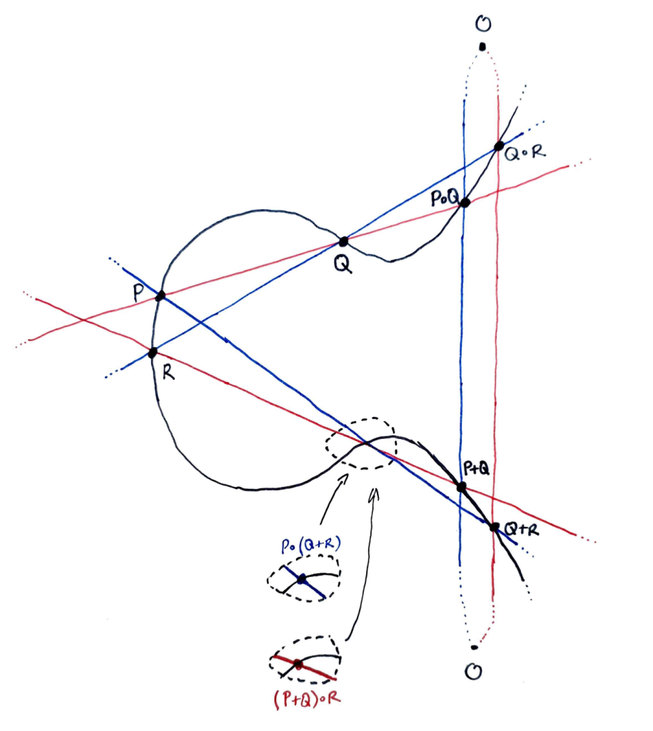
Consider the following diagram. A red line and a blue line intersect the curve $E$ inside the dotted circle. Our goal is to show that these two intersections occur at the same point of $E$ (as indeed they appear to, in the diagram).

Let $l, l’, l^″$ be an enumeration of the red lines, $m, m’, m^″$ an enumeration of the blue lines as follows:


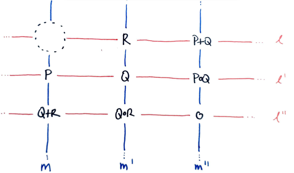
Define cubics $L = l l’ l^″$, $M = m m’ m^″$ (these are the red and blue triangles in the first diagram). Then $E$ and $L$ meet at exactly nine points.

We assume that the eight points $O, P, Q, R, P \circ Q, Q \circ R, P + Q, Q + R$ (in black on both diagrams) are distinct from one another and also from $P \circ (Q + R)$ and $(P + Q) \circ R$ (i.e. the points we are trying to show are equal).

Then $E$ and $L$ have nine points in common (the black points and $(P + Q) \circ R$), and moreover cannot share more than these, since otherwise Bézout’s Theorem (applied to $E$ and each component $l, l’, l^″$ of $L$) would imply that one of these components $l, l’, l^″$ belonged to $E$, thereby contradicting the assumed non-singularity of $E$ (since this implies irreducibility, see note below).

Similarly, $E$ and $M$ share precisely nine points, viz. the black points and $P \circ (Q + R)$. Now $M$ contains eight points (the black points) that are shared by $E$ and $L$, and hence contains also the ninth, by the Cayley-Bacharach Theorem, i.e. $(P + Q) \circ R \in M$.

So $E$ and $M$ share precisely nine points. On the other hand, we’ve shown that they share ten points: the eight black points, $P \circ (Q + R)$, and $(P + Q) \circ R$. Hence, in view of the point distinctness assumptions, the last two points must be equal.

Notes

  • Non-singular curves are irreducible since reducible curves are necessarily singular (since components must intersect by Bézout’s Theorem, and these intersection points are necessarily singularities).

Questions

  • The distinctness assumptions are sufficient in view of Zariski closure?

Further reading

  • Husemöller’s book “Elliptic Curves” (page 51, 2nd edition) proves this, as well as the Cayley-Bacharach theorem itself, along with the corollary of Bézout’s theorem needed for it.
  • Terence Tao’s blog covers the same material as above (and does a much better job of it).
  • Timothy Murphy’s 2016 lecture notes are great.

What does an elliptic curve look like near the point at infinity (the identity)?

The appearance of an elliptic curve from the point of view of the affine $(x,y)$ plane is familiar to us, but leaves us wondering what the curve might look like near the point at infinity (i.e. the identity element $\mathcal{O}$). This is not merely of visual interest, as it allows one to see directly that e.g. a line that is vertical in the $(x,y)$ plane has a pole of order 2 at the identity (even though it also intersects the curve at that point). The divisors of such linear functions play a crucial role in e.g. the computation of the Weil pairing.

Graph embeddings in Hyperbolic Space

I gave a talk last night at the Berlin machine learning meetup on learning graph embeddings in hyperbolic space, featuring the recent NIPS 2017 paper of Nickel & Kiela. Covered are:

  • An illustration of why the Euclidean plane is not a good place to embed trees (since circle circumference grows only linearly in the radius);
  • Extending this same argument to higher dimensional Euclidean space;
  • An introduction to the hyperbolic plane and the Poincaré disc model;
  • A discussion of Rik Sarkar’s result that trees embed with arbitrarily small error in the hyperbolic plane;
  • A demonstration that, in the hyperbolic plane, circle circumference is exponential in the radius (better written here);
  • A review of the results of Nickel & Kiela on the (transitive closure of the) WordNet hypernymy graph;
  • Some thoughts on the gradient optimisation (perhaps better written here).

And here are the slides!

Gradient optimisation on the Poincaré disc

Nickel & Kiela had a great paper on embedding graphs in hyperbolic space at NIPS 2017. They work with the Poincaré ball model of hyperbolic space. This is just the interior of the unit ball, equipped with an appropriate Riemannian metric. This metric is conformal, meaning that the inner product on the tangent spaces on the Poincare ball differ from that of the (Euclidean) ambient space by only a scalar factor. This means that the hyperbolic gradient $\nabla_u$ at a point $u$ can be obtained from the Euclidean gradient $\nabla^E_u$ at that same point just by rescaling. That is, you pretend for a moment that your objective function is defined in Euclidean space, calculate the gradient as usual, and just rescale. This scaling factor depends on the Euclidean distance $r$ of $u$ from the origin, as depicted below:

So far, so good. What the authors then do is simply add the (rescaled) gradient to obtain the new value of the parameter vector, which is fine, if you only take a small step, and so long as you don’t accidentally step over the boundary of the Poincaré disc! A friend described this as the Buzz Lightyear update (“to infinity, and beyond!”). While adding the gradient vector seems to work fine in practice, it does seem rather brutal. The root of the “problem” (if we agree to call it one) is that we aren’t following the geodesics of the manifold – to perform an update, we should really been applying the exponential map at that current point to the gradient vector. Geodesics on the Poincaré disc look like this:

that is, they are sections of circles that intersect the boundary of the Poincaré disc at right angles, or diameters (the latter being a limiting case of the former). With that in mind, here’s a picture showing how the Buzz Lightyear update on the Poincaré disc could be sub-optimal:

The blue vector $\nabla_u$ is the hyperbolic gradient vector that is added to $u$, taking us out of the Poincaré disc. The resulting vector is then pulled back (along the ray with the faintly-marked origin) until it is within the disc by some small margin, resulting in the new value of the parameter vector $u^\textrm{new}$. On the other hand, if you followed the geodesic from $u$ to which the gradient vector is tangent, you’d end up at the end of the red curve. Which is quite some distance away.

Circle circumference in the hyperbolic plane is exponential in the radius: proof by computer game

I recently needed to demonstrate this fact to an audience that I could not assume would be familiar with Riemannian geometry, and it took some time to find a way to do it! You can use the HyperRogue game, which takes place on a tiling of the Poincaré disc. The avatar moves across the Poincaré disc (slaying monsters and collecting treasure) by stepping from tile to tile. It is a pretty impressive piece of software, and you can play it on various devices for small change. Below are four scenes from the game. This image was taken from the interesting paper on HyperRogue by Kopczyński et al., cited at bottom.

As a proxy for proving that the growth rate was exponential, just count the number of tiles that were accessible (starting from the centre tile) in N steps and no less. This gives the sequence 1, 14, 28, 49, 84, 147, 252, 434, 749, … . Plotting this values gives evidence enough.

The authors of the paper do a more thorough job, obtaining a recurrence relation for the sequence and using this to derive the base of the exponential growth (which comes out at about $\sqrt{3}$.

[1] Kopczyński, Eryk; Celińska, Dorota; Čtrnáct, Marek. “HyperRogue: playing with hyperbolic geometry”. Proceedings of Bridges 2017: Mathematics, Music, Art, Architecture, Culture (2017).