Hierarchical Softmax

[These are the notes from a talk I gave at the seminar]

Hierarchical softmax is an alternative to the softmax in which the probability of any one outcome depends on a number of model parameters that is only logarithmic in the total number of outcomes. In “vanilla” softmax, on the other hand, the number of such parameters is linear in the number of total number of outcomes. In a case where there are many outcomes (e.g. in language modelling) this can be a huge difference. The consequence is that models using hierarchical softmax are significantly faster to train with stochastic gradient descent, since only the parameters upon which the current training example depend need to be updated, and less updates means we can move on to the next training example sooner. At evaluation time, hierarchical softmax models allow faster calculation of individual outcomes, again because they depend on less parameters (and because the calculation using the parameters is just as straightforward as in the softmax case). So hierarchical softmax is very interesting from a computational point-of-view. By explaining it here, I hope to convince you that it is also interesting conceptually. To keep things concrete, I’ll illustrate using the CBOW learning task from word2vec (and fasttext, and others).

The CBOW learning task

The CBOW learning task is to predict a word $w_0$ by the words on either side of it (its “context” $C$).

We are interested then in the conditional distribution $P(w|C)$, where $w$ ranges over some fixed vocabulary $W$.

This is very similar to language modelling, where the task is to predict the next word by the words that precede it.

CBOW with softmax

One approach is to model the conditional distribution $P(w|C)$ with the softmax. In this setup, we have:

$$ \hat{y} := P(w|C) = \text{exp}({\beta_w}^T \alpha_C) / Z_C,$$

where $Z_C = \sum_{w’ \in W} {\text{exp}({\beta_{w’}}^T \alpha_C)}$ is a normalisation constant, $\alpha_C$ is the hidden layer representation of the context $C$, and $\beta_w$ is the second-layer word vector for the word $w$. Pictorially:

The parameters of this model are the entries of the matrices $\alpha$ and $\beta$.

Cross-entropy

For a single training example $(w_0, C)$, the model parameters are updated to reduce the cross-entropy $H$ between the distribution $\hat{y}$ produced by the model and the distribution $y$ representing the ground truth:

Because $y$ is one-hot at $w_0$ (in this case, the word “time”), the cross-entropy reduces to a single log probability:
$$ H(y, \hat{y}) := – \sum_{w \in W} {y_w \log \hat{y}_w = – \log P(w_0|C).$$
Note that this expression doesn’t depend on whether $\hat{y}$ is modelled using the softmax or not.

Optimisation of softmax

The above expression for the cross entropy is very simple. However, in the case of the softmax, it depends on a huge number of model parameters. It does not depend on many entries of the matrix $\alpha$ (only on those that correspond to the few words in the context $C$), but via the normalisation $Z_C$ it depends on every entry of the matrix $\beta$. The number of these parameters is proportional to $|W|$, the number of vocabulary words, which can be huge. If we optimise using the softmax, all of these parameters need to be updated at every step.

Hierarchical softmax

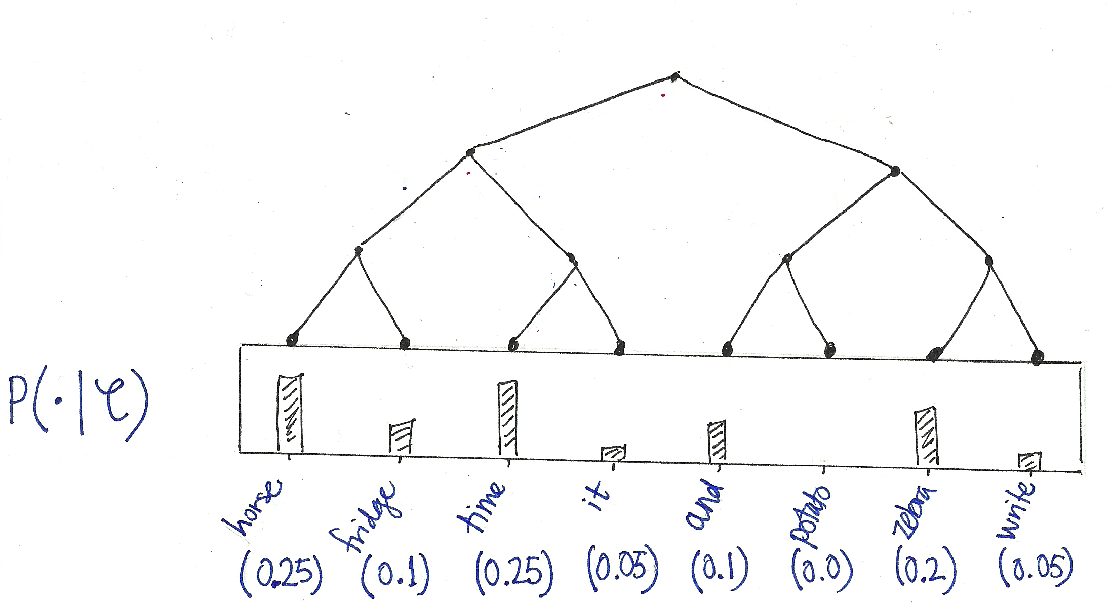
Hierarchical softmax provides an alternative model for the conditional distributions $P(\cdot|C)$ such that the number of parameters upon which a single outcome $P(w|C)$ depends is only proportional to the logarithm of $|W|$. To see how it works, let’s keep working with our example. We begin by choosing a binary tree whose leaf nodes can be made to correspond to the words in the vocabulary:

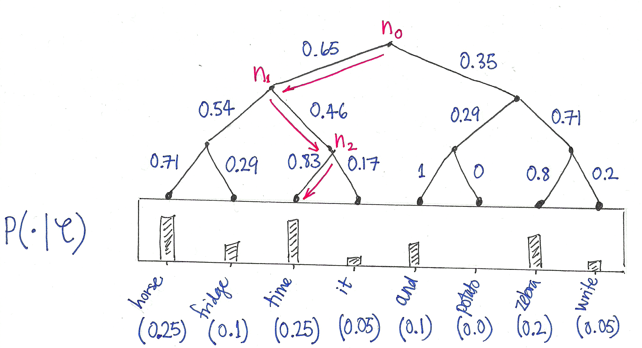
Now view this tree as a decision process, or a random walk, that begins at the root of the tree and descents towards the leaf nodes at each step. It turns out that the probability of each outcome in the original distribution uniquely determines the transition probabilities of this random walk. At every internal node of the tree, the transition probabilities to the children are given by the proportions of total probability mass in the subtree of its left- vs its right- child:

This decision tree now allows us to view each outcome (i.e. word in the vocabulary) as the result of a sequence of binary decisions. For example:
$$ P(\texttt{“time”}|C) = P_{n_0}(\text{right}|C) P_{n_1}(\text{left}|C) P_{n_2}(\text{right}|C),$$
where $P_{n}(\text{right}|C)$ is the probability of choosing the right child when transitioning from node $n$. There are only two outcomes, of course, so:
$$P_{n}(\text{right}|C) = 1 – P_{n}(\text{left}|C).$$
These distributions are then modelled using the logistic sigmoid $\sigma$:
$$ P_{n}(\text{left}|C) = \sigma({\gamma_n}^T \alpha_C),$$
where for each internal node $n$ of the tree, $\gamma_n$ is a coefficient vector – these are new model parameters that replace the $\beta_w$ of the softmax. The wonderful thing about this new parameterisation is that the probability of a single outcome $P(w|C)$ only depends upon the $\gamma_n$ of the internal nodes $n$ that lie on the path from the root to the leaf labelling $w$. Thus, in the case of a balanced tree, the number of parameters is only logarithmic in the size $|W|$ of the vocabulary!

Which tree?

J. Goodman (2001)

Goodman (2001) uses 2- and 3-level trees to speed up the training of a conditional maximum entropy model which seems to resemble a softmax model without a hidden layer (I don’t understand the optimisation method, however, which is called generalised iterative scaling). In any case, the internal nodes of the tree represent “word classes” which are derived in a data driven way (which is apparently elaborated in the reference [9] of the same author, which is behind a paywall).

F. Morin & Y. Bengio (2005)

Morin and Bengio (2005) build a tree by beginning with the “is-a” relationships for WordNet. They make it a graph of words (instead of word-senses), by employing a heuristicFelix, and make it acyclic by hand). Finally, to make the tree binary, the authors repeatedly cluster the child nodes using columns of a tf-idf matrix.

A. Mnih & G. Hinton (2009)

Mnih & Hinto (2009) use a boot-strapping method to construct binary trees. Firstly they train their language model using a random tree, and afterwards calculate the average context vector for every word in the vocabulary. They then recursively partition these context vectors, each time fitting a Gaussian mixture model with 2 spherical components. After fitting the GMM, the words are associated to the components, and this defines to which subtree (left or right) a word belongs. This is done in a few different ways. The simplest is to associate the word to the component that gives the word vector the highest probability (“ADAPTIVE”); another is splitting the words between the two components, so that the resulting tree is balanced (“BALANCED”). They consider also a version of “adaptive” in which words that were in a middle band between the two components are placed in both subtrees (“ADAPTIVE(e)”), which results not in a tree, but a directed acyclic graph. All these alternatives they compare to trees with random associations between leaves and words, measuring the performance of the resulting language models using the perplexity. As might be expected, their semantically constructed trees outperform the random tree. Remarkably, some of the DAG models perform better than the softmax!

Mikolov et al. (2013)

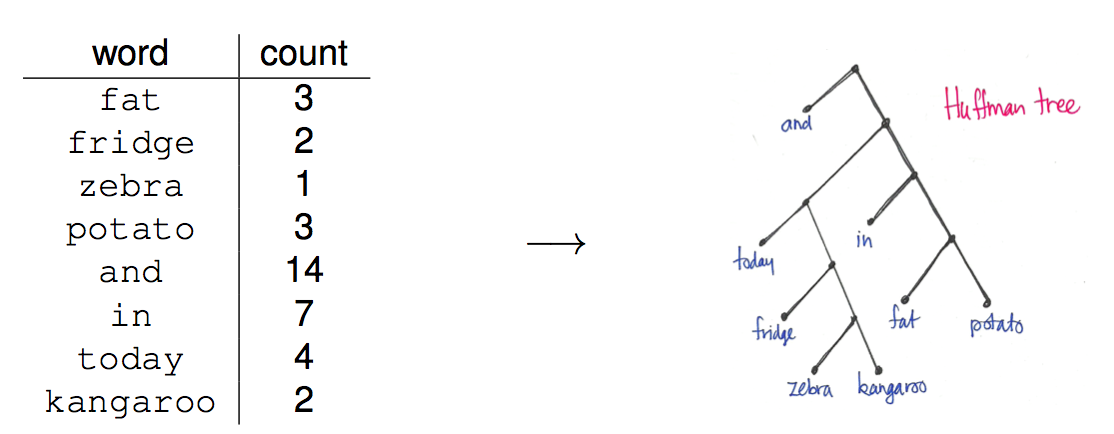
The approaches above all use trees that are semantically informed. Mikolov et al, in their 2013 word2vec papers, choose to use a Huffman tree. This minimises the expected path length from root to leaf, thereby minimising the expected number of parameter updates per training task. Here is an example of the Huffman tree constructed from a word frequency distribution:

What is interesting about this approach is that the tree is random from a semantic point of view.