Recommendation – Building Babylon

20 March 20168 May 2023

Improving Pairwise Learning for Item Recommendation from Implicit Feedback 2014

Steffen Rendle and Christoph Freudenthaler (University of Konstanz), WSDM 2014.

The authors present a modification of the Bayesian Pairwise Ranking (BPR) for implicit feedback (i.e. one class) recommendation datasets in which the negative samples are drawn according both to the models current belief and the user/context in question (“adaptive oversampling“). They show that the prediction accuracy of BPR models trained with adaptive oversampling matches that of BPR models trained with uniform sampling but that convergence is 10x-20x faster.

Consider the problem of recommending items to users (or more generally: contexts, e.g. user on a particular page). The observed data consists then of context-item pairs $(c, i)$, where item $i$ was the choice made in context $c$. The authors work in the context of pairwise learning, which amounts to a binary classification task where context-item-item triples $(c, i, j)$ are labelled as true i.f.f. item $i$ was chosen in context $c$ but item $j$ is not:

where $\hat{y}$ is a scoring function (e.g. the dot product of the context- and the item- latent vectors, for matrix factorisation). It is infeasible to consider all the negative examples $j$, so how should we choose which to consider?

Negative sampling from static distributions

We could draw negative examples from the uniform distribution over all items, or instead from the observed distribution over all items (i.e. by popularity). Both are inexpensive to perform and easy to implement. However:

Uniform sampling tends to yield uninformative samples, i.e. those for which the probability of being incorrectly labelled is very likely already low: popular items are precisely those that appear often as positive examples (and hence tend to be highly ranked by the model), while a uniformly-drawn item is likely to be from the tail of the popularity distribution (so likely lowly ranked by the model).
Sampling according to popularity is demonstrated by the authors to converge to inferior solutions.

The authors point out that these sampling schemes depend neither upon the current context (user) nor the current belief of the model. This contrasts with their own method, adaptive over-sampling.

Adaptive over-sampling

The authors propose a scheme in which the negative samples chosen are those that the model would be likely to recommend to the user in question, according to its current state. In this sense it is reminiscent of the Gibbs sampling used by restricted Boltzmann machines.

Choosing negative samples dependent on the current model and user is computationally expensive if performed in the naive manner. The authors speed this up by working with the latent factors individually, and only periodically re-computing the ranking of the items according to each latent factor. Specifically, in the case of matrix factorisation, when looking for negative samples for a context $c$, a negative sample is chosen by:

sampling a latent factor $l$ according to the absolute values of the latent vector associated to $c$ (normalised, so it looks like a probability distribution);
sampling an item $j$ that ranks highly for $l$. More precisely, sample a rank $r$ from a geometric distribution over possible ranks, then find the item that has rank $r$ when the $l$th coordinates of the item latent vectors are compared.

(We have ignored the sign of the latent factor. If the sign is negative, one choses the rth-to-last ranked item). The ranking of the items according to each latent factor is precomputed periodically with a period such that the extra overhead is independent of the number of items (i.e. is a constant).

Problems with the approach

The samples yielded by the adaptive oversampling approach depend heavily upon the choice of basis for the latent space. It is easy to construct examples of where things go wrong:

Non-negativity constraints would solve this. Regularisation would also deal with this particular example – however regularisation would complicate the expression of the scoring function $\hat y$ as a mixture (since you need to divide though by $Z_c$.

Despite these problems, the authors demonstrate impressive performance, as we’ll see below.

Performance

The authors demonstrate that their method does converge to solutions slightly better than those given by uniform sampling, but twenty times faster. It is also interesting to note that uniform sampling is vastly superior to popularity based sampling, as shown in the diagrams below.

Note that a single epoch of the adaptive oversampling takes approximately 33% longer than a single epoch of uniform sampling BPR.

Implementation

According to the paper, the method is implemented in libFM, a C++ software package that Rendle has published. However, while I haven’t looked exhaustively, I can’t see anything in that package about the adaptive oversampling (nor in Rendle’s other package, MyMediaLite).

What about adaptive oversampling in word2vec?

Word2vec with negative sampling learns a word embedding via binary classification task, specifically, “does the word appear in the same window as the context, or not?”. As in the case of implicit feedback recommendation, the observed data for word2vec is one-class (just a sequence of words). Interestingly, word2vec samples from a modification of the observed word frequency distribution (i.e. of the “distribution according to popularity”) in which the frequencies are raised to the $0.75$th power and renormalised. The exponent was chosen empirically. This raises two questions:

Would word2vec perform better with adaptive oversampling?
How does BPR perform when sampling from a similarly-modified item popularity distribution (i.e. raising to some exponent)?

Corrections

Corrections and comments are most welcome. Please get in touch either via the comments below or via email.

18 March 20168 May 2023

WARP loss for implicit-feedback recommendation

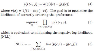
We consider the “Weighted Approximate-Rank Pairwise-” (WARP-) loss, as introduced in the WSABIE paper of Weston et. al (2011, see references), in the context of making recommendations using implicit feedback data, where it has been shown several times to perform excellently. For the sake of discussion, consider the problem of recommending items $i$ to users $u$, where a scoring function $f_u(i)$ gives the score of item $i$ for user $u$, and the item with the highest score is recommended.

WARP considers each observed user-item interaction $(u, i)$ in turn, choses another “negative” item $i’$ that the model believed was more appropriate to the user, and performs gradient updates to the model parameters associated to $u$, $i$ and $i’$ such that the models beliefs are corrected. WARP weights the gradient updates using (a function of) the estimated rank of item $i$ for user $u$. Thus the updates are amplified if the model did not believe that the interaction $(u, i)$ could ever occur, and are dampened if, on the other hand, if the interaction is not surprising to the model. Conveniently, the rank of $i$ for $u$ can be estimated by counting the number of sample items $i’$ that had to be considered before one was found that the model (erroneously) believed more appropriate for user $u$.

Minimising the rank?

Ideally we would like to make updates to the model parameters that minimised the rank of item $i$ for user $u$. Previous work of Usunier (one of the authors) showed that the precision at k was best optimised when the logarithm of the rank was minimised. (to read!)

The problem with the rank is that, while it does depend on the model parameters, this dependence is not continuous (the rank being integer valued!). So it is not possible to speak of gradients. So what is to be done instead? The approach of the authors is to derive a differentiable approximation to the logarithm of the rank, and to minimise this instead.

Derivation: approximating the (log of the) rank

WARP has been shown several times to perform very well for implicit feedback recommendation. However, the derivation of the approximation of the log of the rank used in WARP, as outlined in the WSABIE paper, is nonsense. I can only think that the authors arrived at WARP in another way. Let’s look at it more closely. In the following:

$f_u (i)$ is the score assigned by the model to item $i$ for user $u$.
$L$ is some function that defines the error as a function of the rank. In the WSABIE paper, $L(k) = \sum_{j=1}^k \frac{1}{j}$ is approximately the natural logarithm (for the derivation below, however, it doesn’t matter what $L$ is)

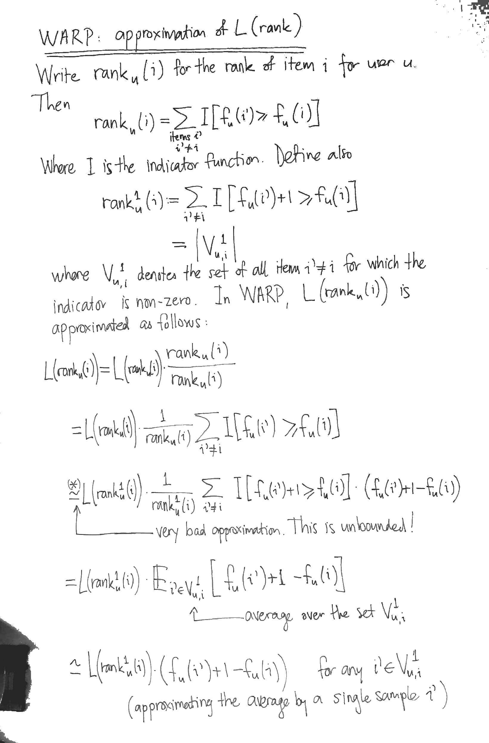
warp derivation The most obvious problem with the derivation is the approximation marked with an asterix (*). At this step, the authors approximate the indication function $I[x > y]$ by $I[x > y] \cdot (x – y + 1)$. While the latter is familiar as the hinge loss from SVMs, it is (begin unbounded!) a dreadful approximation for the indicator $I[x > y]$. It seems to me that the sigmoid of the difference of the scores would be a much better differentiable approximation to the indicator function.

To appreciate why the derivation is nonsense, however, you have to notice that the it has nothing to do with $L$. That is, the derivation above would yield an approximation for $L$, whatever $L$ happened to be, even a constant function.

Optimisation

WARP considers each observed interaction $(u, i)$ in turn, repeatedly sampling items $i’$ from the uniform distribution over all items until it finds one in $V_{u, i}^1$, i.e. until it finds an item $i’$ whose score for the user $u$ is at worst 1 less than the score of the observed interaction. For this triple $(u, i, i’)$, it performs gradient updates to minimise:

$\displaystyle L( \text{rank}_u^1 (i) ) \cdot (f_u (i’) + 1 – f_u (i))$

The naive approach to computing $\text{rank}_u^1 (i)$ is to calculate all the scores for the given user in order to determine the rank of the item $i$. WARP performs a nice trick to do much better: it estimates $\text{rank}_u^1 (i)$ by counting how many candidate negative items $i’$ it had to consider before finding one in $V_{u, i}^1$. This yields

$\displaystyle \text{rank}_u^1 (i) \approx \frac{\text{total number of items} – 1}{\text{number of i’ we had to draw}}$

However it is still the case that $L(\text{rank}_u^1 (i))$ is not differentiable. So when we compute the gradients, this quantity has to be treated as a constant. Thus it simply becomes a weighting applied to the gradient of the difference of the scores (hence the name WARP, I guess).

WARP optimises for item to user recommendations

With its negative sampling technique, WARP optimises for recommending items to a user. For instance, the problem of recommending users to items (so, transposing the interaction matrix) is not trained for. I wonder if some extra uplift could be obtained by training for both problems simultaneously.

Normalising for the total number of items

With the optimisation stated as above, the learning rate will need to be re-tuned for datasets that have different numbers of items, since the gradient weighting $L( \text{rank}_u^1 (i) )$ is ranges from $L(0)$ to $L(\text{total number items})$. It would make more sense to weigh the gradient updates by:

$\displaystyle \frac{L( \text{rank}_u^1 (i) )}{L(\text{total number items})}$

which ranges between 0 and 1.

Implementations

There are two implementations of WARP for recommendation that I know of, both in Python:

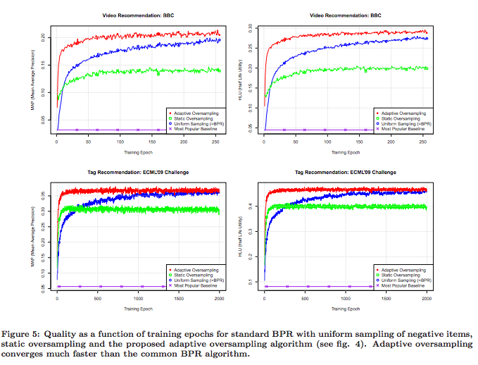
LightFM, written by Maciej Kula. Works well. Also implements BPR with uniform sampling and WARP k-OS (which I’ve not investigated yet).
MREC, written by Levy and Jack at Mendeley, has a matrix factorisation recommender trained using WARP. I’ve not tried this one out yet.

References

Jason Weston, Samy Bengio and Nicolas Usunier, Wsabie: Scaling Up To Large Vocabulary Image Annotation, 2011, (PDF).

26 January 20168 May 2023

Metadata Embeddings for User and Item Cold-start Recommendations

Maciej Kula (Lyst)
CBRecSys 2015 (arxiv)

Kula presents a model for cold start recommendation, which he calls “LightFM”. Users and items are considered as sets of binary features. For example:

$\text{alice} = \{ \text{domain}:\text{gmail} \}$

$\text{itemXYZ} = \{\text{description}:\text{pleated}, \text{description}:\text{skirt}, \text{tag}:\text{chanel} \}.$

Each of these features (e.g. each tag, each word and each email domain) corresponds to a parameter vector and a bias term. A user vector (or item vector) is then the sum of the vectors associated to its constituent features. Similarly, a user (item) bias term is just the sum of the bias terms associated to its features.

The probability $\hat{r}(u, i)$ of an interaction between a user $u$ and an item $i$ is modelled as the sigmoid of the dot product of the user vector and the item vector, along with the bias terms associated with the user and the item:

$\hat{r}(u, i) := \sigma (vec(u) \cdot vec(i) + bias(u) + bias(i))$

The model is trained on a set $S_{+}$ of user-item pairs observed as having interacted, and on a set $S_{-}$ of user-item pairs that were not observed to have interacted (in the case of implicit feedback recommendation) or to have interacted negatively (in the case of explicit feedback recommendation). Specifically, these interactions and non-interactions are assumed independent and the likelihood

$\displaystyle L = \prod_{(u, i) \in S_{+}} \hat{r}(u,i) \cdot \prod_{(u, i) \in S_{-}} (1 – \hat{r}(u,i))$

is then maximised using stochastic gradient descent and with adaptive per-parameter learning rates determined by Adagrad.

Trivial featurisation gives matrix factorisation

Note that users (or items) can be featurised trivially using their ids. We create one user feature for each user id, so that the user-feature matrix is the identity matrix. In this case, we have a separate parameter vector for each user. If we do this for both users and items, then the model is just a (sigmoid-) factorisation of the user-item interaction matrix. This is then the case of Johnson’s logistic matrix factorization.

Evaluation

Performance is evaluated on MovieLens for explicit feedback recommendation and on CrossValidated (one of the StackExchange websites) for implicit feedback recommendation. In both cases, warm- and cold-start scenarios are tested. Warm start is tested by holding out interactions in such a way that every item and every user is still represented in the training interaction data. Cold start is tested by holding out all interactions for some items. Model accuracy is measured by considering each user in the set of test interactions, considering the binary classification task of labelling each item as having been interacted with or not and then measuring the area under the curve of the associated ROC curve. The mean is that taken over all users in the test set.

LightFM seems to perform well in both cold and warm start scenarios.

Engineering Notes

Kula included some interesting notes on the production use of LightFM at Lyst. Training is incremental with model state stored in the database.

Implementation and Examples

Available on GitHub and extensively documented. Written in Cython. In addition to the logistic loss used above, Bayesian Personalised Ranking and WARP are supported.

26 August 20158 May 2023

A Bayesian Personalised Ranking Example: Factor Models for Recommending Given Names

Immanuel Bayer and Steffen Rendle

ECML PKDD Discovery Challenge 2013 (offline track).

This paper provides an interesting example of using factorisation machines for implicit feedback via the Bayesian personalised ranking (BPR) optimisation criterion.

The challenge was to recommend first names (e.g. to soon-to-be parents). Participants were provided with the browsing history of users on the name selection website Nameling. So the items to be recommended are names.

Users are considered together with their browsing history, consisting of the name they looked at last and the list of all the names they looked at up to the time $t$ in question. The combination of a user (in this complete sense) at time $t$ and a candidate name is vectorised as follows:

The (order 2) factorisation machine assigns a score to the combination as follows:

where $p$ is the rank of this vectorisation, $w_0 \in \mathbb{R}$, $w \in \mathbb{R}^p$ and $V \in \mathbb{R}^{p \times k}$ are model parameters to be learned. These parameters are learned via stochastic gradient ascent of the following pair-wise learning objective:

where $D$ is the set of (user u, time t, name n) tuples where u has browsed n before time t, $N$ is the set of all possible names and $\sigma$ is the sigmoid function. Only a single name is chosen from $N \setminus \{ n \}$ for each update. These negative samples are drawn according to their estimated rank (this part is quite difficult to do efficiently).

In the above, we have purposefully omitted the “prefix smoothing” step, since we are mainly interested in the a simple factorisation machine example. The details are in the paper.

Remarks
This recommender did very well in the challenge. However, I don’t find the examples given in the paper very impressive (though I have not seen the examples given by others). My suspicion is that the FM approach is very strong, but that there is no good way to make first name recommendations using the provided dataset. A more effective dataset would be e.g. first name x product interaction on a large e-commerce site. This would do a much better job of capturing the social meaning of names, but could go out of date very quickly.

11 August 20158 May 2023

Collaborative Filtering for Implicit Feedback Datasets

Hu, Koren and Volinsky (AT&T, Yahoo!), 2008.

A well-written paper.

PDF

The authors give a good description of the distinctions between explicit and implicit feedback datasets, pointing out in particular that:

implicit feedback data is inherently noisy, since a user might decide that they do not like an item after viewing it — interaction does not necessarily indicate interest.
the numerical value in explicit feedback indicates preference whereas in the implicit case indicates confidence.

The authors describe their model as being based on SVD, but this is not accurate, since they weight squared difference summands in the cost function according to a confidence value (which is proportional to the number of interactions for that user-item pair).

The input matrix is the user-item matrix.

Optimisation is via alternating least squares.

Their evaluation metric is percentile rank based.

Their model, which we’ll call “weighted SVD” (they speak of “confidence intervals”) compares favourably with the baseline popularity method and also with an old-school item-based neighbourhood method, in terms of the expected percentile rank (Figure 1). Interestingly, the differences are less marked when the probability that a desired item is in the top (say) 1% is considered (Figure 2).

The unweighted SVD on the user-item matrix is shown to perform terribly, with a significant but insufficient improvement obtained with regularisation.

11 August 20158 May 2023

Logistic Matrix Factorization for Implicit Feedback Data

Christopher Johnson, Spotify, 2014

PDF

A new matrix factorisation model for behavioural recommendation in the case of implicit feedback is presented.

User-item interactions are encoded in a non-negative interaction matrix. The question as to whether a user-item interaction occurred is then treated as a problem of binary classification. User-item pairs for which an interaction has occurred are regarded as positive outcomes with confidence in constant proportion to the value in the interaction matrix, while the absence of an interaction is regarded as a negative outcome. This binary classification is task is then leveraged to train user- and item-vectors. These vectors reside in dually paired spaces. The dot-product of the vectors, combined with user- and item- bias terms, is then fed into the sigmoid function. What we are really doing is looking for a low-rank approximation to a bilinear form via the sigmoid function.

Confidence values (proportional to the values in the interaction matrix) are used as powers of their corresponding factor in the maximum likelihood function. The constant proportion that defines the confidence values from the interaction matrix is a tuning parameter, but is typically chosen so that the positive outcomes balance the negative outcomes in total confidence. Thus the likelihood function is weighed according to the entries of the interaction matrix. The weighted likelihood function is then maximised using alternating gradient ascent. This optimisation is batch. Negative sampling can be used to speed up convergence, and the confidence parameter is decreased proportionally.

Evalutation
They use a fractional rank type metric to evaluate performance at each iteration. For each user, the interaction probability is computed for each item, and the rank of the target item in this list is determined. This is then averaged over a set-aside collection of user-item pairs. Given that batch gradient descent is used, this is not prohibitively expensive.

The author reports that this logistic matrix factorisation model performs better in low rank than the implicit MF model of Koren et al 2008, though both give a similar fractional rank in high ranks.

Implementation
A very basic implementation in Python is available. The implementation uses AdaGrad to dynamically chose a step size at each iteration, just as is described in the paper. The paper mentions a Spark or Hadoop based implementation, but I couldn’t find this published anywhere.

23 July 20158 May 2023

A Graph-Based Method for Combining Collaborative and Content-Based Filtering

Phuong, Thang and Phuong (all from the Posts and Telecommunications Institute of Technology, Vietnam), 2008.

PDF obtainable here.

The authors present a recommendation system that incorporates user ratings of items (they work in the explicit rating context) and item-feature relations. The approach is graphical. Effectively, two weighted graphs with non-negative weights are constructed, network propagation is performed on both independently and the two resulting scorings are combined in a weighted sum. The first graph is directed represents user-item preference via the item features (where the user-feature preferences are computed heuristically from the given ratings and item-feature associations); thus in this graph all paths from user to item have length 2. The second graph is undirected and represents the purely positive user ratings of items and excludes the item features. The two graphs capture the content- and collaborative- aspects of the recommendation problem, respectively.

I find the approach lacks unity and is too heuristic. The unity suggested by the user/item/feature graph of Figure 1 is merely pictorial, since network propagation is actually performed on the two graphs described above (which are derived from this unified graph) separately. The two separate graphs are constructed heuristically, and this removes any claim the approach might have had to necessity.

The more obvious, unified, approach (network propagation on the user/item/feature graph) is unavailable here since the user-item associations may be negative. This would not be the case if the feedback were implicit (e.g. purchases). For this reason I will be interested to read the paper of Huang et al. cited by the authors – perhaps they use just such an approach. Furthermore, Huang et al. experiment with different network propagation algorithms (in this paper, a modification of an algorithm by Weston et al. is used).

The MovieLens dataset is used in the evaluations, which demonstrate the superiority of the authors approach over a purely content, a purely collaborative and a simple hybrid approach that merges the result sets of collaborative filtering and content recommendation computed separately.

Paper is clearly written.

22 July 20158 May 2023

HybridRank: A Hybrid Content-Based Approach to Mobile Game Recommendations

Chow, Foo and Manai (all at Group Digital Life, Singtel, Singapore) 2014.

PDF.

The authors consider a personalised PageRank on a graph whose vertices represent items for recommendation and whose edge weights are determined by feature overlap (where features are e.g. category, tag). In order to incorporate collaborative information into the computation, they define the “teleport vector” (or “reset vector”) for a user to be the sum over all items they’ve interacted with of the corresponding rows of the behavioural item x item matrix (they call these “user correlation matrices”, somewhat confusingly).

This is a nice advance from “ItemRank” for incorporating item meta information into the recommendation process. In contrast to ItemRank, the authors work in the context of implicit feedback data. However, I think that the approach could be made more elegant by considering the users and tags (for example) as additional vertices in the graph – the reset vector would then just be the one-hot vector singling out the vertex corresponding to the user receiving the recommendations.

The authors carry out an enormous user survey and an impressive live production test to demonstrate the performance of their approach.

22 July 20158 May 2023

ItemRank: A Random-Walk Based Scoring Algorithm for Recommender Engines

Marco Gori and Augusto Pucci, 2007 (from the IJCAI conference proceedings).

PDF.

The authors consider an application of PageRank to recommendation in the case where explicit ratings are available. The vertices of the graph represent items to be recommended, and the weight of the edge between any two vertices is proportional to the number of users that have interacted with both the corresponding items (thus the explicit ratings are not incorporated into the graph itself). To obtain recommendations for a particular user, the “reset-” (or “teleport-“) vector of is set to be the explicit ratings given by the user (0 is used for the absence of a rating), PageRank is run and then resulting importances are used to rank the items.

It seems to me that this set-up would be more sensible in contexts where the behavioural data was implicit (e.g. user looked at particular item) rather that explicit (user gave a particular rating to a particular item) – in the explicit context the use of the value 0 for the absence of rating can not be motivated.

The authors test their approach on the MovieLens dataset.

As the authors themselves note, PageRank had been used for personalised (more generally, deliberately biased) recommendation before their work (e.g. Haveliwala “Topic sensitive Pagerank”, 2002). The novelty here lies in the construction of the graph from the user-item interaction matrix.

10 July 201518 May 2023

PageRank meets vectorial representations – "Ranking on Data Manifolds"

I came across this paper when following up on ideas I had when reading about TextRank for summarising documents. It is short, well written and very interesting, and was authored by Zhou, Weston, Gretton, Bousquet and Schölkopf (all then at the Max Planck Institute for Biological Cybernetics, Tübingen) in 2004. (PDF).

The authors consider the problem of ranking objects by relevancy to one or more query objects in the case where the objects have a vectorial representation. This is done using the PageRank algorithm on a graph in which the vertices represent the objects and the edges weights are computed using e.g. an RBF kernel (or normalised dot-product, if the vectors are non-negative).

One advantage of this approach is that it generalises naturally to multiple query vectors. The query vectors are simply treated as a complete list of possible (re)starting points for the PageRank random walk. This contrasts with the typical PageRank case, where all pages are possible starting points. Note that this list of starting points need not be binary — it can rather be a probability distribution over the objects representing user preference.

The PageRank approach is shown to perform much better than Euclidean nearest neighbours search on real world data sets (MNIST digits and newsgroup posts are considered). In both cases, the datasets have labels. The query data points are chosen from a single class, and the ranking problem is treated as one of binary classification, i.e. finding the distinguishing the objects of the same class from those of all other classes. The ranking is used to calculate a ROC curve, and the area under this curve is used as a performance measure.

The evaluation considers the case of multiple query vectors, as well. The Euclidean nearest neighbours, in the multiple query vector case, are aggregated by taking the minimal distance to a query vector (i.e. “disjunctively”).

The PageRank method is visually contrasted with the Euclidean nearest neighbours case using the MNIST data set. Below are the 99 best ranked results in PageRank case (left) and the Euclidean case (right) (99 = 10 x 10 – 1 query). Not only does the left panel contain no threes, but the twos are more homogeneous.

The graph that the authors construct is not complete. Rather, edges are added, beginning with those most heavily weighted (but excluding self-loops) until the graph is connected. For example, in the case of the two sickle moons:

Hyperparameters
An RBF kernel function is used in some cases to define the edge weighting between nodes (see step 2 of the algorithm). Note that the variance $\sigma$ of the RBF kernel needs to be fitted using cross-validation. This is no problem for labelled datasets like MNIST, but would be problematic for e.g. the sickle moons data.

It’s not a random walk
Note that, due to the “symmetric normalisation” that is applied to the affinity matrix $W$ (see step 3 of the algorithm), this is not a random walk — the columns of the normalisation $S$ do not sum to 1, so the iterative procedure of step 4 will not map probability distributions to probability distributions. Given that we only want to rank the nodes, not derive a probability distribution over them, this is not necessarily a problem.

Why symmetric normalisation? Dengyong was kind to explain the motivation for this (via correspondence). This normalisation was used in order to avoid over-emphasising points in high density regions, and because it is the normalised graph Laplacian (I haven’t looked into this). Dengyong added that these reasons were not strong, and that other alternatives should be investigated.

Corrections to the paper
There are some mistakes in the paper. In particular, there is a problem with Theorem 2, pointed out by begab on reddit when I shared this post. Begab points out that $DU \neq DU$. The problem is larger than this, in fact, since the claim that the steady state of a PageRank random walk on a connected, undirected graph does not hold. There is the following counterexample, for instance.

Questions

Who has taken this research further?
In both of the cases considered, the vector representations of the objects are rather poor (pixel on/off and tf-idf). How much better is this approach if dimension reduction is first applied to the vectors?