The following is intended as an introduction to finite fields for those with already some familiarity with algebraic constructions. It is based on a talk given at our local seminar.
A finite field is simply a field with a finite number of elements. An example of a finite field that should already be familiar is $\mathbb{Z} / p \mathbb{Z}$, the integers modulo a prime $p$, which in the context of field theory is more commonly denoted $\mathbb{F}_p$. But what other finite fields exist? In this post, we’ll construct a finite field $\mathbb{F}_{p^n} = GF(p^n)$ of size $p^n$ for any prime $p$ and positive integer $n$, and additionally prove that, up to isomorphism, these are all the finite fields.
(Note that another common notation for $\mathbb{F}_{p^n}$ is $GF(p^n)$ – the “GF” stands for “Galois field”).
$\mathbb{F}_p$ is a field
Firstly, let’s take a moment to show why $\mathbb{F}_p$ is a field. It is clearly is a commutative ring with 1, so it remains to see why every non-zero element $a$ has an inverse. We need to find an element $x$ such that $ax \equiv 1 \mod p$. The Extended Euclidean Algorithm provides a way to find such a $x$. The algorithm takes two positive integers $a, b$ and returns integer coefficients that linearly combine $a$ and $b$ to yield their GCD, i.e. such that $ax + by = \gcd(a, b)$. Take $b=p$. Since $p$ is prime and $a$ is not zero, $\gcd(a, p) = 1$. The Euclidean algorithm therefore yields $x$ and $y$ such that $ax + py = 1$, which means $ax \equiv 1 \mod p$. Hence, $x$ is the multiplicative inverse of $a$.
This same argument will be recycled below in our construction of extension fields.
The characteristic of a field
The characteristic of a field $K$ is the smallest positive integer $p$ such that $p \cdot 1 := 1 + \cdots + 1$ ($p$ times) equals $0$ in $K$. In other words, it is the order of the additive group generated by the element $1$.
If $K$ is finite, then it is clear that such a $p$ must exist. Moreover, $p$ must be prime. For supposing that $p$ factorized, as say $p=rs$ with $1 < r, s < p$, it would follow that \begin{equation}\label{ZD}\tag{ZD}(r \cdot 1) (s \cdot 1) = 0,\end{equation} while at the same time, by minimality of the characteristic, we’d have that neither of the multiplicands $r\cdot 1$, $s \cdot 1$ were themselves zero. To arrive at a contradiction, either note that you’ve constructed zero divisors in a field, or instead use that fact that $r \cdot 1$ (being non-zero) has an inverse, multiply both sides of \eqref{ZD} by that inverse and note that this would force $s \cdot 1 = 0$, a contradiction.
(A similar argument shows that $\mathbb{Z} / m\mathbb{Z}$ is not a field if $m$ is not prime).
If no positive integer $p$ exists such that $p \cdot 1 = 0$, the characteristic is defined to be zero (this is the case for $\mathbb{Q}, \mathbb{R}, \mathbb{C}$, for example).
The prime subfield
A subfield of a field is simply a subset which is itself a field (with the same $1$ and $0$). The prime subfield of a field $K$ is the subfield generated by $1$ and is the smallest subfield contained in $K$. If the characteristic of $K$ is a prime number $p$, then the prime subfield is (a copy of) the field $\mathbb{F}_p$. If the characteristic of $K$ is zero, then the prime subfield is isomorphic to the field of rational numbers $\mathbb{Q}$.
Of course, the prime subfield could be the entire field!
Any finite field has size a prime power, and that prime is its characteristic
Let $K$ be a finite field of characteristic $p$, and identify $\mathbb{F}_p$ with the prime subfield of $K$. Now let’s forget some of the structure of $K$ and just consider $K$ as a vector space over the field $\mathbb{F}_p$. The vector space axioms are indeed satisfied, since elements of $K$ can be added together, and multiplied by scalars (i.e. elements of $\mathbb{F}_p$) in a way that is distributive and associative – all of this just follows from the field axioms.
Now let $n \geq 1 $ be the dimension of $K$ as a vector space over $\mathbb{F}_p$. If you chose a basis for $K$, it would have length $n$, and every element of $K$ would have a unique expression as a linear combination of the basis with coefficients in $\mathbb{F}_p$. Moreover, every such expression would be an element of $K$. There are $p^n$ such expressions, so $| K | = p^n$.
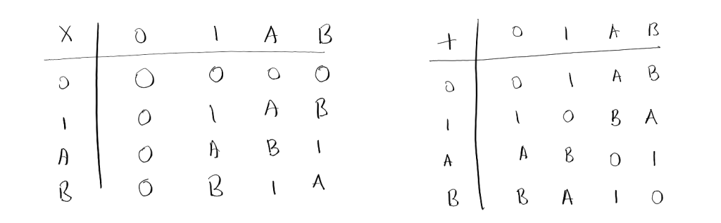
Example: there is precisely one field with four elements
While we will indeed construct $\mathbb{F}_{p^n}$ for every prime $p$ and $n >0$, let’s first do the simplest possible example beyond the more familiar fields $\mathbb{F}_p$: let’s “manually” construct a field $\mathbb{F}_4$ with four elements. Indeed, we’ll see that there is only one such field, up to isomorphism.
Firstly, note that $\mathbb{F}_4$ has characteristic 2 (by the preceding section), and hence has $\mathbb{F}_2$ as its prime subfield. So there are only two “new” field elements. Call them $A, B$, so that $\mathbb{F}_4 = \{ 0, 1, A, B \}$. Note that the four elements must all be pairwise non-equal, or the field is too small. Now, try to fill in the multiplication table for this new field, using the fact that the non-zero elements of a field (in our case: $1, A, B$) must form a group under multiplication. This implies that each element can appear at most once in each row and column. You’ll see that there is only one way to do this!
Similarly, try filling in the addition table, this time using the fact that the field is a group under addition, as well as $A + A = A \cdot (1 + 1) = A \cdot 0 = 0$ (similarly for $B$). There is only one possible addition table!
Below, we’ll construct this same finite field (and many others) but in a more sophisticated manner.
Polynomial prerequisites
Polynomial division
Given two polynomials $f, g \in K[x]$, $f \ne 0$, we can perform polynomial division to write $g(x) = q(x)f(x) + r(x)$ for some unique $q, r \in K[x]$ such that $ \text{deg}(r) < \text{deg}(f)$. Call $q$ the quotient and $r$ the remainder. This is analogous to the division algorithm for integers.
Roots correspond to linear factors
A polynomial $f(x)$ has a root $\lambda$ if and only if it is divisible by the linear polynomial $(x – \lambda)$. This can be seen using polynomial division: for if $f(x)$ is divided by $(x – \lambda)$, then the remainder is $f(\lambda)$. Hence, $f(\lambda) = 0$ if and only if the remainder is zero, which means $f(x)$ is divisible by $(x – \lambda)$.
Aside: a finite field is never algebraically closed
While this subsection has no relevance to the construction below, it is too nice to omit!
Recall that a field $K$ is said to be algebraically closed if every non-constant polynomial $f(x) \in K[x]$ has a root in $K$. For example, $\mathbb{C}$ is algebraically closed, while $\mathbb{R}$ is not. Now if $K$ is a finite field, form the polynomial $$f(x) = (\prod_{\lambda \in K} (x – \lambda) ) + 1 $$ and notice that $f(\lambda) \ne 0$ for any $\lambda \in K$. Thus $K$ can not be algebraically closed.
Irreducible polynomials
An irreducible polynomial over a field $K$ is a non-constant polynomial that cannot be factored into the product of two non-constant polynomials over $\mathbb{F}$. Irreducibles of degree three or lower are easy to find: any factorization must involve a linear factor, and these can be detected by evaluating the polynomial (as discussed above).
Exercise 1: Verify that, over $\mathbb{F}_2$, the polynomial $x^2 + x + 1$ is the unique quadratic irreducible.
Exercise 2: (Again over $\mathbb{F}_2$) show that $x^3 + x + 1$ and $x^3 + x^2 + 1$ are the unique cubic irreducibles.
A stepping stone: constructing new fields from old
Let $K$ be any field (not necessarily finite) and let $f \in K[x]$ an irreducible polynomial of degree $n$. Write $ K_{(f)} = K[x] / f K[x]$ for the quotient of the ring $K[x]$ by the ideal generated by $f$. Then $K_{(f)}$ is itself a ring with $1$. Let $\pi : K[x] \to K_{(f)}$ be the surjection of rings that comes from the quotient construction, i.e. that maps any polynomial $g$ to its coset $g + f K[x]$.
Just as the elements of $\mathbb{Z} / p \mathbb{Z}$ are enumerated by remainders after integer division by $p$, the elements $g + f K[x]$ of $K_{(f)}$ can be enumerated by remainders $r(x)$ of polynomial division of $g(x)$ by $f(x)$: if $g=qf + r$, then $\pi(g) = \pi(r)$. If $K$ is indeed finite, this immediately tell us that $|K_{(f)}| = |K|^n$, since there are $|K|$ possibilities for each of the $n = \text{deg} (f)$ coefficients of $r(x)$.
There is moreover an extended Euclidean algorithm for polynomials, and (analogous to our argument for $\mathbb{Z} / p \mathbb{Z}$) this can be used to demonstrate that every non-zero element of $K_{(f)}$ has an inverse. For if $a$ is such an element, than there exists a $g \in K[x]$ with $\pi(g) = a$, and we have that $g$ is not divisible by $f$, since $a \ne 0$. Thus, the greatest common divisor of $f$ and $g$ (which is defined to be the monic polynomial of maximal degree dividing both $f$ and $g$), in view of the irreducibility of $f$, must be $1$. The extended Euclidean algorithm therefore yields polynomials $s, t \in K[x]$ such that $sf + tg = 1$, and applying $\pi$ to both sides of this equation shows that $\pi(t) = \pi(g)^{-1}$, i.e. $\pi(t)$ is the inverse of $a = \pi(g)$.
We’ve thus shown that $K_{(f)}$ is a field. Indeed, it has $K$ as a subfield, and so $K \subset K_{(f)}$ is a field extension. It is, in fact, quite a special field extension – the polynomial $f$, which was irreducible over $K$, has a root $K_{(f)}$, namely $\pi(x)$. To see this, first note that $\pi$ is a $K$-linear map. Then:
$$ f (\pi (x)) = \sum_i f_i (\pi(x))^i
= \sum_i f_i \pi (x^i)
= \pi \left(\sum_i f_i x^i \right)
= \pi (f (x))
= 0.$$
In summary, given a field $K$ and an irreducible $f \in K[x]$ of degree $n$, we’ve constructed an extension field of $K$ in which $f$ has a root!
Note that we’d have achieved our goal of constructing a field with $p^n$ elements if we knew that there was an irreducible polynomial of degree $n$ over $\mathbb{F}_p$. But we don’t know this at this stage. Nonetheless, the above construction is the crucial ingredient, as we’ll see below.
Exercise 3: Verify that the complex numbers $\mathbb{C}$ can be constructed from the real numbers $\mathbb{R}$ in this way, using the irreducible quadratic $f(x) = x^2 + 1 \in \mathbb{R}[x]$. In particular, you should recover the familiar formulae for the real and complex parts of the multiplication of two complex numbers from multiplication in $K_{(f)}$. (For a worked solution, see here).
Exercise 4: Carry out the above construction for $K = \mathbb{F}_2$ and the irreducible $f(x) = x^2 + x + 1 \in K[x]$, and check that you obtain the field with four elements (which we constructed earlier in manual fashion).
Exercise 5: (continuing the example of the previous exercise) Show that both roots of $f$ are obtained ($\pi(x)$ is one of them, which is the other?). Though we won’t use (or show) this here, it turns out that this is always true if $K$ is finite, then $f$ will factor completely into linear factors over the extension field $K_{(f)}$. You can cycle through the roots by applying the Frobenius automorphism.
Existence of a splitting field
Suppose $K$ is a field (not necessarily finite) and $h \in K[x]$ a non-constant polynomial. A splitting field for $h$ is a field $L$ extending $K$ (so $K \subset L$) over which $h$ splits as a product of linear factors, and that is minimal with the property, i.e. if $L’$ with $K \subset L’ \subset L$ is another such field, then $L’ = L$.
We show here that splitting fields exist (a special case of which will be the last ingredient in our construction of the finite fields).
We proceed iteratively. $h$ has a unique expression as a product of irreducibles over $K$. If this expression consists only of linear factors, then stop. If not, choose a non-linear (i.e. degree > 1) irreducible factor $f$, and construct the field $K_{(f)}$ as above. Considering $h \in K_{(f)}[x]$, we see that $h$ has at least one more linear factor than before. Repeat this process, each time replacing $K$ by $K_{(f)}$ where $f$ is one of the remaining non-linear irreducible factors of $h$. Since polynomials have finite degree, this process which terminate with a field $\hat L$ over which $h$ factors linearly. Now take the smallest subfield $L \subset \hat L$ over which $h$ factors linearly (such a field is uniquely determined, since the intersection of any two subfields with this property will again be a subfield with this property). Then we have constructed a splitting field for $h$.
Construction of a field with $p^n$ elements
Finally! Using the construction of the previous section, let $L$ be a splitting field of $h(x) = x^{p^n} – x \in \mathbb{F}_p [x]$. So $\mathbb{F}_{p^n} \subset L$. Now let $L’ = \{ \lambda \in L \,|\, h(\lambda) = 0 \}$. It remains to show that $L’$ is a field and $|L’| = p^n$.
To see that $L’$ is a field, first note that $0, 1 \in L$ are both roots of $h$, so $0, 1 \in L’$. Now simply show that $L’$ is closed under addition, multiplication, and inversion. Only addition is not immediate: for this, you need to use that the binomial coefficients $\binom{p^n}{k}$ vanish in characteristic $p$ whenever $0 < k < p^n$ (which follows from the definition of the binomial coefficient in terms of factorials, c.f. here). Thus $L’$ is a field.
Finally, note that $|L’|$ is equal to the number of distinct roots of $h$. The polynomial $h$ has degree $p^n$, but perhaps there are repeated roots? There are not. If a root $\lambda$ was repeated, then $(x – \lambda)^2$ would divide $h$. But if this were the case, then $(x – \lambda)$ would divide its derivative $\frac{dh}{dx}$ (this follows immediately from the product rule for differentiation). But direct calculation shows that $\frac{dh}{dx} = -1$ (in characteristic $p$), and so $h$ can have no repeated roots. Hence $|L’| = p^n$, and we have constructed a field with $p^n$ elements!
Extension: these are all the finite fields
In the previous section, we constructed a splitting field $L’$ for the polynomial $h(x)$ and showed that it had $p^n$ elements. But could there be multiple, non-isomorphic fields of size $p^n$? There can not, as we see below. We need this uniqueness up to isomorphism in order to be able to sensibly speak of “the field $\mathbb{F}_{p^n}$ with $p^n$ elements”!
Suppose that $K$ is some other field with $|K| = p^n$, so $\mathbb{F}_{p} \subset K$. Then the set of all non-zero elements of $K$ is a multiplicative group of size $p^n – 1$. Thus for any non-zero $\lambda \in K$, we have that $\lambda^{p^n – 1} = 1$, or, put differently, that $\lambda^{p^n} – \lambda = 0$, i.e. $h(\lambda) = 0$! Note that this holds also for $\lambda = 0$, so we’ve shown that every element of $K$ is a root of $h$. Since $|K| = p^n = \text{deg}(h)$, it follows that $h$ factors linearly over $K$, and that $K$ is a minimal extension of $\mathbb{F}_p$ with this property since $h$ has no repeated factors (as seen in the previous section). Thus $K$ is a splitting field for $h$ as well, i.e. all fields of size $p^n$ are splitting fields for $h$.
Splitting fields are unique up to isomorphism in the sense detailed below. This statement is trivial if, as some authors do, you chose to consider only fields inside of a fixed algebraic closure of $\mathbb{F}_p$. If, like me, you would prefer not to do this, you might proceed as follows.