GloVe: Global Vectors for Word Representations

Pennington, Socher, Manning, 2014.
PDF

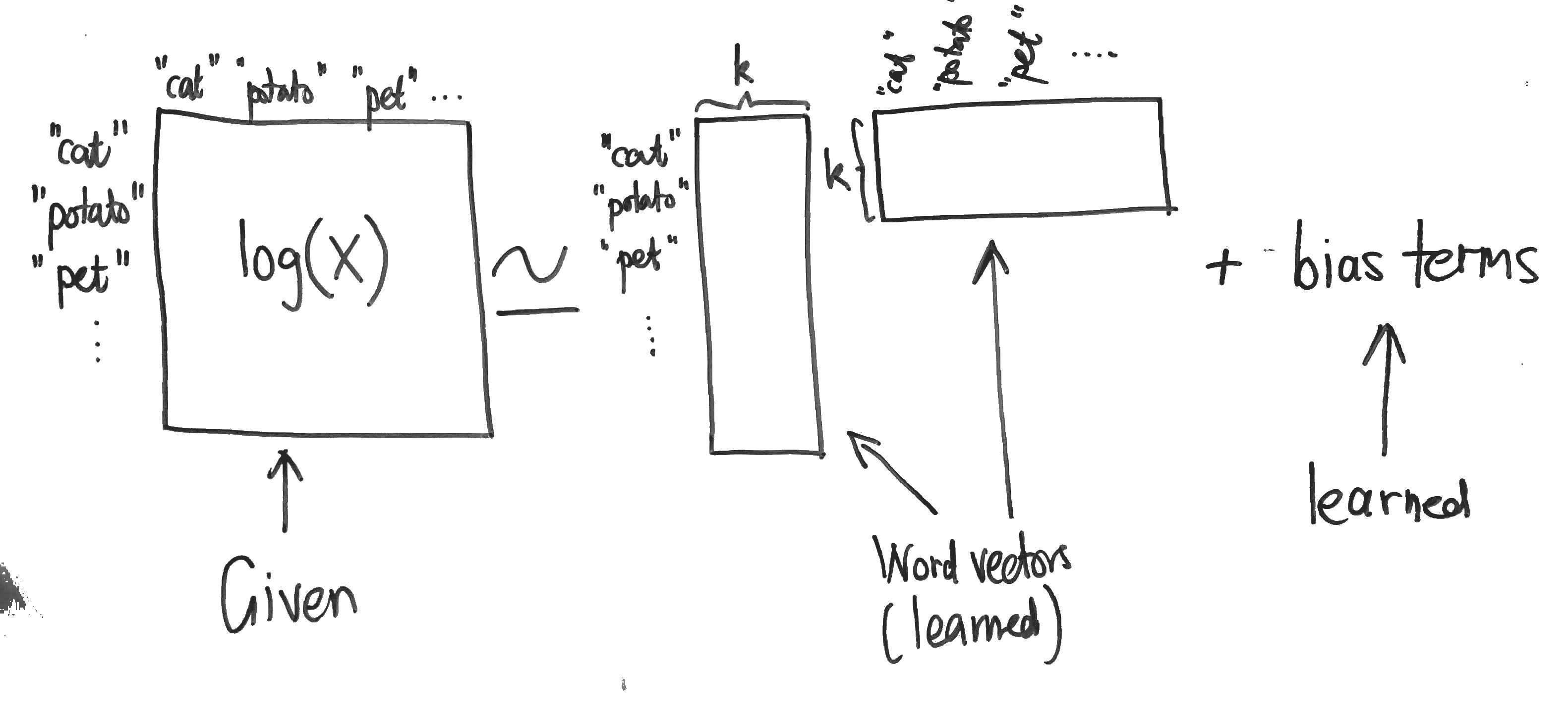
GloVe trains word embeddings by performing a weighted factorisation of the log of the word co-occurrence matrix. The model scales to very large corpora (Common Crawl 840B tokens) and performs well on word analogy tasks.

Model
The cost function is given by:

$\displaystyle \sum_{i, j = 1}^V f(X_{i,j}) (u_i^T v_j + b_i + c_j – \text{log} X_{i,j})^2$

where:

  • $V$ is the size of the vocabulary,
  • $X$ denotes the word co-occurrence matrix (so $X_{i,j}$ is the number of times that word $j$ occurs in the context of word $i$)
  • the weighting $f$ is given by $f(x) = (x / x_{\text{max}})^\alpha$ if $x < x_{\text{max}}$ and $1$ otherwise,
  • $x_{\text{max}} = 100$ and $\alpha = 0.75$ (determined empirically),
  • $u_i, v_j$ are the two layers of word vectors,
  • $b_i, c_j$ are bias terms.

Note that the product is only over pairs $i, j$ for which $X_{i,j}$ is non-zero. This means that GloVe (in contrast to word2vec with negative sampling) trains only “positive samples” and also that we don’t have to worry about the logarithm of zero.

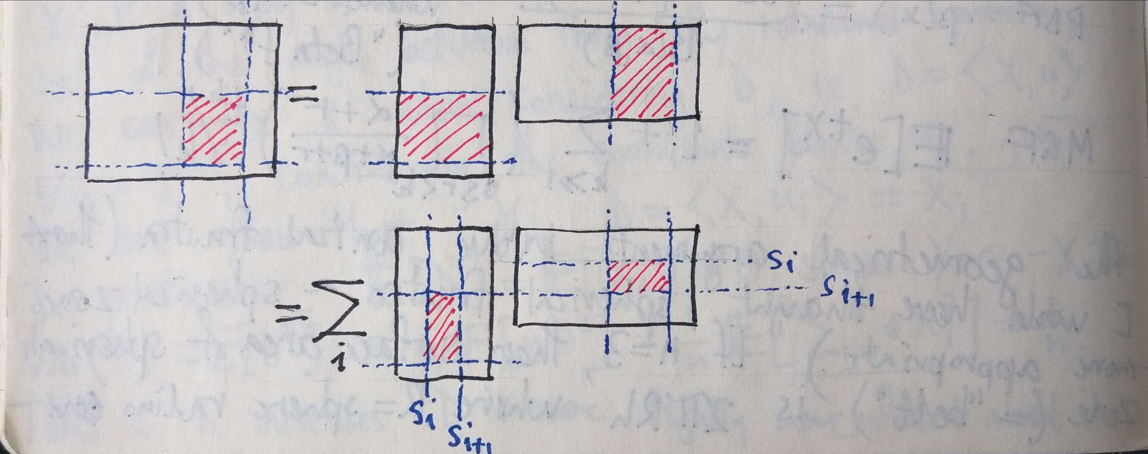
This is essentially just weighted matrix factorisation with bias terms:

glove-matrix-factorisation

Note that in the implementation (see below), the $X_{i,j}$ are not raw co-occurrence counts, but rather the accumulated inverse distance between the two words, i.e.

$\displaystyle X_{w, w’} := \sum_{\text{windows containing\ } w, w’} (\text{distance between\ } w, w’)^{-1}.$

I am fairly sure that the implementation of Adagrad is incorrect. See my post to the forum.

The factor weighting f

The authors go to some trouble to motivate the definition of this cost function (section 3).  The authors note that many different functions could be used in place of their particular choice of $f$, and further that their $\alpha$ coincides with that used by word2vec for negative sampling. I can’t see the relevance of the latter, however (in word2vec, the $0.75$th power it is used to define the noise distribution; moreover powering a value in the range $[0, 1]$ has a very different effect to powering a value in the range $[0, 100]$).

glove-weighting-function

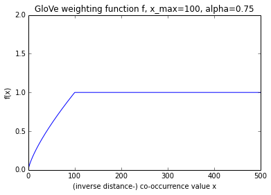
Graphing the function (see above) hints that it might have been specified more simply, since the non-linear region is in fact almost linear.

A radial window size of 10 is used. Adagrad is used for optimisation.

Word vectors
The resulting word embeddings ($u_i$ and $v_j$) are unified via a direct sum of their vector spaces.

The cosine similarity is used to find the missing word in word similarity tasks. It is not stated if the word vectors were normalised before forming the arithmetic combination of word vectors.

Source code
The authors take the exemplary step of making the source code available.

Evaluation and comparison with word2vec
The authors do a good job of demonstrating their approach, but do a scandalously bad job of comparing their approach to word2vec. This seems to reflect a profound misunderstanding on the part of the authors as to how word2vec works. While it has to be admitted that the word2vec papers were not well written, it is apparent that the authors made very little effort at all.

The greatest injustice is the comparison of the performance of GloVe with an increasing number of iterations to word2vec with an increasing number of negative samples:

The most important remaining variable to control
for is training time. For GloVe, the relevant
parameter is the number of training iterations.
For word2vec, the obvious choice would be the
number of training epochs. Unfortunately, the
code is currently designed for only a single epoch:
it specifies a learning schedule specific to a single
pass through the data, making a modification for
multiple passes a non-trivial task. Another choice
is to vary the number of negative samples. Adding
negative samples effectively increases the number
of training words seen by the model, so in some
ways it is analogous to extra epochs.

Firstly, it is simply impossible that it didn’t occur to the authors to simulate extra iterations through the training corpus for word2vec by simply concatenating the training corpus with itself multiple times. Moreover, the authors themselves are capable programmers (as demonstrated by their own implementation). The modification to word2vec that they avoided is the work of ten minutes.

Secondly, the notion that increasing the exposure of word2vec to noise is comparable to increasing the exposure of GloVe to training data is ridiculous. The authors clearly didn’t take the time to understand the model they were at pains to criticise.

While some objections were raised about the evaluation performed in this article and subsequent revisions have been made, the GloVe iterations vs word2vec negative sample counts evaluation persists in the current version of the paper.

Another problem with the evaluation is that the GloVe word vectors formed as the direct sum of the word vectors resulting from each matrix factor. The authors do not do word2vec the favour of also direct summing the word vectors from the first and second layers.

Links

Perpendicularity and dimension

We show below that vectors drawn uniformly at random from the unit sphere are more likely to be orthogonal in higher dimensions.

In information retrieval and other areas besides, it is common to use the dot product of normalised vectors as a measure of their similarity. It can be problematic that the similarity measure depends upon the rank of the representation, as it does here — it means, for example, that similarity thresholds (for relevance in a particular situation) need to be re-calibrated if the underlying vectorisation model is retrained e.g. in a higher dimension.

Question
Does anyone have a solution to this? Is there a (of course, dimension dependent) transformation that can be applied to the dot product values to arrive at some dimension independent measure of similarity?

I asked this question on “Cross Validated”. Unfortunately, it has attracted so little interest that it has earned me the “tumbleweed” badge!

For those interested in the distribution of the dot products, and not just the expectation and the variance derived below, see this answer by whuber on Cross Validated.

Marginal and Conditional Distributions of the Multivariate Gaussian

This is the standard, elementary arithmetic proof that the marginal and conditional distributions of the multivariate Gaussian are again Gaussian with parameters expressible in terms of the covariance matrix of the original Gaussian. We use the block multiplication of matrices.

I was surprised by how much work is required to show this, and feel moreover that the proof (while correct) fails to offer any intuitive understanding. Is there not a higher-level, co-ordinate free proof of this important result, perhaps one that uses characteristic properties of multivariate Gaussians?

Update: I received an answer to this question on Cross Validated from whuber. He uses a generative definition: the multivariate Gaussians are precisely the affine transformations of tuples of standard (mean zero, unit-variance) one-dimensional Gaussians. Using this definition, it follows quickly that the conditional and marginal distributions must be multivariate Gaussian.

Block Multiplication of Matrices

(We needed this to derive the conditional distribution of a multivariate Gaussian).

Consider a matrix product $AB$. Partition the two outer dimensions (i.e. the rows of $A$ and the columns of $B$) and the one inner dimension (i.e. the columns of $A$ and the rows of $B$) arbitrarily. This defines a “block decomposition” of the product $AB$ and of the factors $A, B$ such that the blocks of $AB$ are related to the blocks of $A$ and $B$ via the familiar formula for components of the product, i.e.

$(AB)_{m,n} = \sum_s A_{m,s} B_{s,n}$.

Pictorially, we have the following:

blockmultnmatrices

Arithmetically, this is easy to prove by considering the formula above for the components of the product. The partitioning of the outer dimensions comes for free, while the partitioning of the inner dimension just corresponds to partitioning the summation:

$(AB)_{m,n} = \sum_s A_{m,s} B_{s,n} = \sum_i \sum_{s_i \leq s \leq s_{i+1}} A_{m,s} B_{s,n}$.

Zooming out to a categorical level, we can see that there is nothing peculiar about this situation. If, in an additive category, we have three objects $X, Y, Z$ with biproduct decompositions, and a chain of morphisms:

$X \xrightarrow{\varphi_B} Y \xrightarrow{\varphi_A} Z$

then this “block decomposition of matrices” finds expression as a formula in $\text{End}(X, Z)$ using the injection and projection morphisms associated with each biproduct factor.