Graph embeddings in Hyperbolic Space

I gave a talk last night at the Berlin machine learning meetup on learning graph embeddings in hyperbolic space, featuring the recent NIPS 2017 paper of Nickel & Kiela. Covered are:

  • An illustration of why the Euclidean plane is not a good place to embed trees (since circle circumference grows only linearly in the radius);
  • Extending this same argument to higher dimensional Euclidean space;
  • An introduction to the hyperbolic plane and the Poincaré disc model;
  • A discussion of Rik Sarkar’s result that trees embed with arbitrarily small error in the hyperbolic plane;
  • A demonstration that, in the hyperbolic plane, circle circumference is exponential in the radius (better written here);
  • A review of the results of Nickel & Kiela on the (transitive closure of the) WordNet hypernymy graph;
  • Some thoughts on the gradient optimisation (perhaps better written here).

And here are the slides!

Gradient optimisation on the Poincaré disc

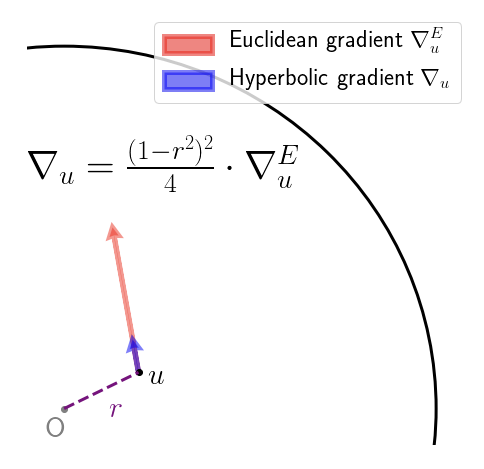
Nickel & Kiela had a great paper on embedding graphs in hyperbolic space at NIPS 2017. They work with the Poincaré ball model of hyperbolic space. This is just the interior of the unit ball, equipped with an appropriate Riemannian metric. This metric is conformal, meaning that the inner product on the tangent spaces on the Poincare ball differ from that of the (Euclidean) ambient space by only a scalar factor. This means that the hyperbolic gradient $\nabla_u$ at a point $u$ can be obtained from the Euclidean gradient $\nabla^E_u$ at that same point just by rescaling. That is, you pretend for a moment that your objective function is defined in Euclidean space, calculate the gradient as usual, and just rescale. This scaling factor depends on the Euclidean distance $r$ of $u$ from the origin, as depicted below:

So far, so good. What the authors then do is simply add the (rescaled) gradient to obtain the new value of the parameter vector, which is fine, if you only take a small step, and so long as you don’t accidentally step over the boundary of the Poincaré disc! A friend described this as the Buzz Lightyear update (“to infinity, and beyond!”). While adding the gradient vector seems to work fine in practice, it does seem rather brutal. The root of the “problem” (if we agree to call it one) is that we aren’t following the geodesics of the manifold – to perform an update, we should really been applying the exponential map at that current point to the gradient vector. Geodesics on the Poincaré disc look like this:

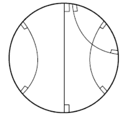
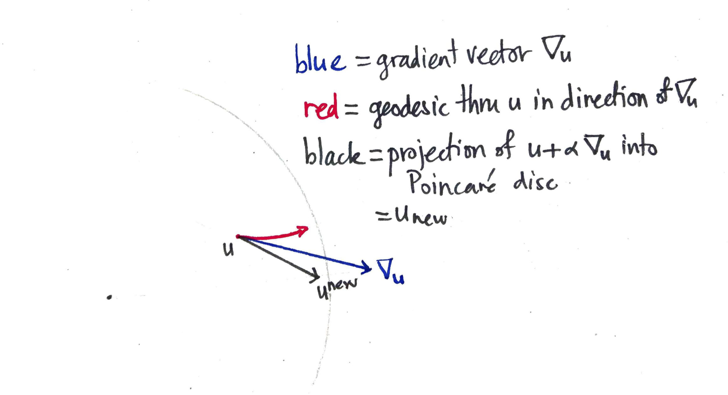
that is, they are sections of circles that intersect the boundary of the Poincaré disc at right angles, or diameters (the latter being a limiting case of the former). With that in mind, here’s a picture showing how the Buzz Lightyear update on the Poincaré disc could be sub-optimal:

The blue vector $\nabla_u$ is the hyperbolic gradient vector that is added to $u$, taking us out of the Poincaré disc. The resulting vector is then pulled back (along the ray with the faintly-marked origin) until it is within the disc by some small margin, resulting in the new value of the parameter vector $u^\textrm{new}$. On the other hand, if you followed the geodesic from $u$ to which the gradient vector is tangent, you’d end up at the end of the red curve. Which is quite some distance away.

Circle circumference in the hyperbolic plane is exponential in the radius: proof by computer game

I recently needed to demonstrate this fact to an audience that I could not assume would be familiar with Riemannian geometry, and it took some time to find a way to do it! You can use the HyperRogue game, which takes place on a tiling of the Poincaré disc. The avatar moves across the Poincaré disc (slaying monsters and collecting treasure) by stepping from tile to tile. It is a pretty impressive piece of software, and you can play it on various devices for small change. Below are four scenes from the game. This image was taken from the interesting paper on HyperRogue by Kopczyński et al., cited at bottom.

As a proxy for proving that the growth rate was exponential, just count the number of tiles that were accessible (starting from the centre tile) in N steps and no less. This gives the sequence 1, 14, 28, 49, 84, 147, 252, 434, 749, … . Plotting this values gives evidence enough.

The authors of the paper do a more thorough job, obtaining a recurrence relation for the sequence and using this to derive the base of the exponential growth (which comes out at about $\sqrt{3}$.

[1] Kopczyński, Eryk; Celińska, Dorota; Čtrnáct, Marek. “HyperRogue: playing with hyperbolic geometry”. Proceedings of Bridges 2017: Mathematics, Music, Art, Architecture, Culture (2017).