While there is famously no “royal road to geometry”, I believe that there is a royal road to understanding the wonderful logUp, a lookup argument from Starkware’s Shahar Papini and Polygon’s Ulrich Haböck. We’ll take this royal road here. This is significantly more direct than the approach taken in the two papers. The advantage of the exposition of the papers is that the thought processes that led to the final formulation are apparent (which is appreciated). The advantage of the exposition here is that it is formulated with the benefit of hindsight and ignores the historical development. Consequently (I hope!), you’ll get to the heart of the matter faster.
The setup for any lookup argument is a “table” $t$ of values that are permitted, and a “witness column” $w$ consisting of values to be checked. Both the table and witness column are multisets, typically represented as one-dimensional arrays of field elements, where repetition of an element in the array is used to represent multiplicity of that element in the multiset. The goal a lookup is to demonstrate (with high probability) that all of the witness values appear in the table, or equivalently, that considered as sets (i.e. ignoring multiplicities), the witness is a subset of the table, i.e. \begin{equation}\textstyle \tag{Subset}\label{Subset} \forall i \ \exists j \ :\ w_i = t_j .\end{equation} The table and witness are typically different lengths, but we’ll assume for simplicity that they are both powers of two, say $$ \textstyle w = (w_i)_{i=0, \dots, 2^M – 1} \qquad t = (t_j)_{j=0, \dots 2^N – 1}, $$ for some $M, N \geq 0$.
What’s wrong with the naive approach to lookups?
To see what’s truly wonderful about logUp, it’s crucial to see what’s wrong with a “naive” lookup argument. A typical lookup argument (not logUp) would show \eqref{Subset} by exhibiting, for each table entry $t_j$, a non-negative integer $m_j \geq 0$ and then showing (via random evaluation) that the following polynomial equality holds \begin{equation}\tag{Naive}\label{Naive} \textstyle \prod_{i=0}^{2^M – 1} (X – w_i) = \prod_{j=0}^{2^N – 1} (X – t_j)^{m_j}.\end{equation} To see why this is problematic, consider how the exponents on the right hand side will be computed in circuit using addition and multiplication gates. Before anything else, $X$ is replaced with a random field element $\alpha$ (in pursuit of Schwartz-Zippel). Then, for each $(\alpha-t_j)$, all of the powers \begin{equation} \textstyle (\alpha – t_j)^{2^0}, (\alpha – t_j)^{2^1}, (\alpha – t_j)^{2^2}, \dots, (\alpha – t_j)^{2^M – 1}\end{equation} need to be computed by repeated squaring. These powers are then combined to obtain $(\alpha – t_j)^{m_j}$: $$ \textstyle (\alpha – t_j)^{m_j} = \prod_{k=0}^{M – 1} \left( b_k^{(j)} (\alpha – t_j)^{2^k} + (1 – b_k^{(j)}) \right),$$ where $m_j = \sum_{k=0}^{M – 1}{b_k^{(j)} 2^k}$ is the binary decomposition of $m_j$ into bits $b_k^{(j)}$, for $j=0, \dots M-1$. And that’s the problem: not only do the multiplicities $m_j$ need to be provided to the circuit as inputs, but so do their binary decompositions! This is an order $M$ (=log of witness length) blow up in the number of circuit inputs. All inputs have to be committed to, and that’s expensive.
What’s so great about logUp?
LogUp demonstrates that $w \subset t$ by exhibiting, for each table entry $t_j$, a field element $m_j \in \mathbb F_q$ such that that the following “logUp identity” holds: \begin{equation}\tag{LogUp}\label{LogUp} \textstyle \sum_{i=0}^{2^M – 1} \frac{1}{X – w_i} = \sum_{j=0}^{2^N – 1} \frac{m_j}{X – t_j}. \end{equation} Setting aside for a moment the meaning of the inverse polynomial summands, we can see already why logUp is great. The multiplicities are not non-negative integers, but rather field elements, and using them in circuit involves just scalar multiplication! In particular, no binary decomposition of the multiplicities is required, resulting in significantly fewer inputs to be committed to (in contrast to the naive approach outlined above).
The logarithmic derivative
The logarithmic derivative of a function is just the derivative of its logarithm. If you apply this transformation to both sides of naive lookup equation \eqref{Naive}, you’ll see you get the logUp equation \eqref{LogUp}. To do this, you’ll need to work symbolically, treating polynomials as formal objects (not functions, see below). While this connection between the two equations is conceptually pleasing (and important for understanding where logUp came from), it is worth noting that proof of the soundness of the logUp approach doesn’t use the logarithmic derivative. See Lemma 5 (which relies on Lemma 4) of the 2022 logUp paper, or see below for an alternative proof.
The logUp identity is an equation in the field of fractions
Before attempting to show that the logUp identity is equivalent to the subset relation, let’s pause to think about where the logUp identity \eqref{LogUp} “lives”.
Recall that polynomials are formal arithmetic combinations of field elements and an indeterminate (so e.g. $X^2 \ne X$ in $\mathbb{F}_2[X]$, even though they coincide as functions $\mathbb{F}_2 \to \mathbb{F}_2$, because they are distinct formal sums; c.f. here). There is no danger in making this distinction. Any equality between two polynomials is also an equality between their corresponding polynomial functions (since evaluation at any point is a ring homomorphism).
The field of fractions $\mathbb{F}(X)$ is similarly a formal object, consisting of pairs of polynomials $(p, q)$, where $q \ne 0$, that are considered up to an equivalence that mimics that of fractions, i.e. $(p,q) \sim (p’, q’)$ if and only if $pq’ = p’q$. They can be formally added and multiplied in the way that seems natural if one writes $p/q$ for $(p,q)$ (if unfamiliar, have a play and convince yourself that all is okay).
The logUp identity \eqref{LogUp} is an equality in the field of fractions $\mathbb{F}(X)$.
How to show \eqref{LogUp}: Schwartz-Zippel for the field of fractions
Let $p(X), q(X)$ be the polynomials given by
$$\frac{p(X)}{q(X)} = \left(\sum_{i=0}^{2^M – 1} \frac{1}{X – w_i} \right) \ -\ \left(\sum_{j=0}^{2^N – 1} \frac{m_j}{X – t_j} \right),$$ where $q(X)$ is the obvious product of all the denominators (i.e. with repetition). To show that the logUp identity \eqref{LogUp} holds, we need to show that $p(X) / q(X) = 0 / 1$ in $\mathbb{F}(X)$, i.e. that $p(X) = 0$ and $q(X) \ne 0$. Random evaluation (a.k.a. Schwartz-Zippel) can be used to show both of these simultaneously (w.h.p.). There are two small caveats: (i) if you’re unlucky and you hit a root of $q(X)$, you’ll need to resample, and (ii) you need to take the inverse of the evaluation of $q(X)$ as an input to the circuit to show that that evaluation is indeed non-zero in circuit.
For randomly sampled $\alpha \in \mathbb{F}$, if $$ \alpha \ne w_i \ \ \forall i, \quad \wedge \quad \alpha \ne t_j \ \ \forall j, \quad \wedge \quad \sum_i \frac{1}{\alpha – w_i} = \sum_j \frac{m_j}{\alpha – t_j}$$ then (since evaluation at any $\alpha$ is a ring homomorphism) $$ p(\alpha) = 0 \quad \wedge \quad q(\alpha) \ne 0$$ from which it follows (w.h.p.) that $\frac{p(X)}{q(X)} = 0$, which implies \eqref{LogUp}.
The logUp relation \eqref{LogUp} is equivalent to the subset relation \eqref{Subset}
As mentioned, this is shown in Lemma 5 and 4 of the 2022 paper. We show it here in a different way.
One direction of implication is trivial: if \eqref{Subset}, then \eqref{LogUp} clearly holds. Note that this is irrespective of the characteristic of the field (not so for the converse, as we’ll see).
We prove the converse statement (i.e. \eqref{LogUp} implies \eqref{Subset}) via the contrapositive, but for this we need the assumption $2^M < \text{char}(\mathbb F)$, i.e. that the witness length is bounded by the characteristic of the field. Suppose that \eqref{Subset} does not hold. Then there exists some $i_0$ such that $w_{i_0} \ne t_j$ for all $j$. Let $I$ denote the set of all indices $i$ such that $w_i = w_{i_0}$, and write $K = |I|$. Note that $K < 2^M < \text{char}(\mathbb F)$. Let $p(X), q(X)$ be as in the previous section. Since $q(X) \ne 0$, to show that \eqref{LogUp} is not satisfied, it suffices to show that $p(X) \ne 0$. Straightforward calculation shows that $p(X)$ can be written in the form $$ p(X) = (X – w_{i_0})^{K-1} \varphi(X) + (X – w_{i_0})^{K} \psi(X)$$ where $$\textstyle \varphi(X) = K \left( \prod_{i \not \in I} (X – w_i) \right) \left( \prod_{j} (X – t_j) \right)$$ and $\psi(X)$ is a polynomial (which polynomial doesn’t matter). By $K-1$ applications of the product rule for differentiation (as per usual, we differentiate polynomials symbolically), we see that $$\textstyle p^{(K-1)}(w_{i_0}) = (K-1)! \, \varphi(w_{i_0}).$$ Recalling that $K$ is bounded by the characteristic, we see by inspection that $\varphi (w_{i_0}) \ne 0$ and consequently (by the same fact) that $p^{(K-1)}(w_{i_0}) \ne 0$. Thus $p^{(K-1)}(X) \ne 0$, and so $p(X) \ne 0$, and we’re done.
Fractional sumcheck via the GKR protocol
We saw above that, in order to show \eqref{LogUp} w.h.p., we need to show that $$\tag{Eval}\label{Eval} \sum_i \frac{1}{\alpha – w_i} = \sum_j \frac{m_j}{\alpha – t_j}$$ for some random $\alpha \in \mathbb{F}$. This is just a relationship in the field. To show it, the authors describe “fractional sumcheck”, which amounts to separately reducing each side to a single fraction, and then showing that these two fractions are equal.
The reduction of each side of the equation is expressed as a layered arithmetic circuit to which the GKR protocol can be applied. Imagine we want to reduce a sum $$ \sum_{b \in \mathcal B^N} \frac{p(b)}{q(b)},$$ where $\mathcal B = \{0,1\}$ and $p$ and $q$ are functions $\mathcal B^N \to \mathbb{F}$. Note that e.g. the right hand side of \eqref{Eval} can be written in this form by replacing the indices $j=0,\dots,2^N – 1$ of the multiplicities $m$ and the table $t$ with bitstrings $b \in \mathcal B^N$ and defining the functions $p$ and $q$ to give the numerators and denominators of the summands. Now define $N+1$ functions
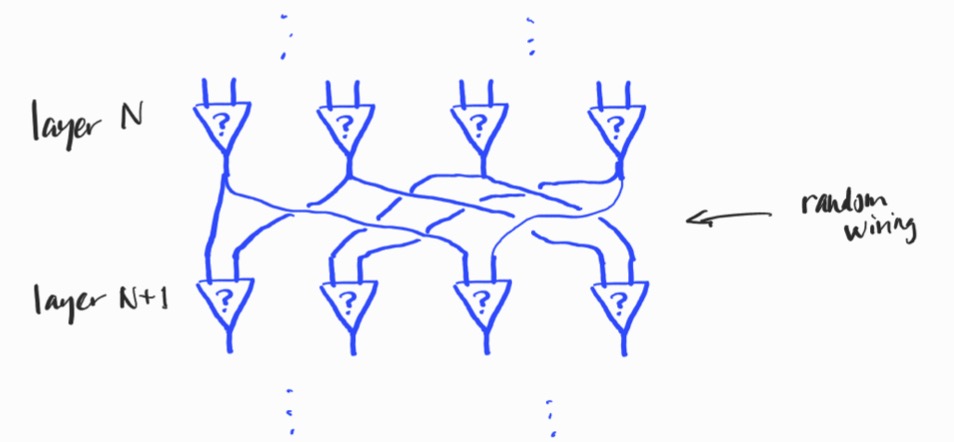
$$ p_k, q_k : \mathcal B^k \to \mathbb{F}, \qquad 0 \leq k \leq N,$$ by $p_N := p$, $q_N := q$ and $$ p_k (b) := p_{k+1}(0b) q_{k+1}(1b) + p_{k+1}(1b)q_{k+1}(0b),$$ $$q_k (b) := q_{k+1}(0b) q_{k+1}(1b)$$ for all $b \in \mathcal B^k$, where e.g. $1b$ denotes the bitstring of length $k+1$ obtained by prefixing $b$ with a $1$. Then the desired single fraction is the ratio of field elements (i.e. functions on $\mathcal B^0$) $p_0 / q_0$. Do the same for the other side of the equation, obtaining $p’_0 / q’_0$, and then check both sides are equal via $pq’ – qp’=0$ and $q \ne 0$, $q’ \ne 0$ (these last two are shown using the inverses of $q$ and $q’$, taken as inputs). The above defines a layered arithmetic circuit with wiring that is regular in the sense of the GKR protocol. This allows the satisfaction of the circuit to be efficiently verified without needing to materialize (or commit to) any of the intermediate values. For more on the GKR protocol, check out Thaler’s book, or instead this blogpost by Remco Bloemen.
The case of batch witness columns
LogUp works just as well for a batch of witness columns. We haven’t made that explicit in the above (contrary to the presentation of the papers) because it suffices to simply concatenate the witness columns and sum up their multiplicities.
Other works using the logarithmic derivative for lookups
As described in the introduction to the 2022 logUp paper, there was both existing and concurrent work using the logarithmic derivative for lookup arguments (they are on the reading list!):
- Bulletproof++ (Eagen et al., 2022);
- A blog post from ZK research (Roh et al., 2022);
- flookup (Gabizon & Khovratovich, 2022);
- Cached quotients (Eagen at al., 2022).
Thanks
Thank you to the exceptional team at Modulus Labs, Georg Wiese, Victor Sint Nicolaas, Hamish Ivey-Law and Ulrich Haböck for helpful discussions and suggestions (any errors are my own).
References
2023 paper
- Improving logarithmic derivative lookups using GKR (Papini & Haböck)
- Talk at PSE